How We Made a Robot
Ideation & Outreach
CAVEMAN started out as a group of ambitious electrical and computer engineering students wanting to make a cool mechatronic/robotic project. Most of the members had worked together beforehand with successful outcomes, so the next step was something a bit bigger. The first initial idea was a Moon rover that would navigate and build roads on the moon using regolith sintering and brick laying. Outreach and resources on that front were a bit limited despite Pitt building up its space academics and research. Outreach from Carnegie Robotics Laboratory were more fruitful in problem discovery, leading us to look into cave and mine robotics. They also introduced us to the realm of Photogrammetry, which made up a large part of our mapping pipeline.

Carnegie Robotics Laboratory also referred us to Mine Vision Sytems, giving us insight on methods and technologies that we utilized in our final system, such as RTABMAP. Working with Pitt's Civil & Environmental Engineering Department, we learned more about the current issues with caves, such as their inaccurate and outdated mapping, giving us more motivation in this problem space. This resulted in our transition from a space rover into a cave rover, equipping us with better access to testing facilities and reducing the constraints to ensure higher project feasibility in the single semester timeframe. Working with the vice chair of the ECE department as our advisor, he steered us clear of other ideas that come with much higher complication and logistics, like drones, and also provided us with additional resources, like an NVIDIA Jetson Nano, to smoothly aid our robotics journey. More outreach in the ECE department helped us work out power and motor considerations, and our connections with the Bioengineering Department secured us a private workspace.

Despite many successes in outreach, a lot of avenues bore no fruit. We tried working with MSHA, CMU's NREC, and many others in the mining and robotics community in Pittsburgh, but we were declined; while they would have been very helpful, this had very little hindrance on our end result besides providing a few more areas to explore and map.
Design
When designing this rover, we started from the top, with functional constraints first. Since our robot is intended to be used in caves and mines, considering all the environmental hazards and technological limitations was extremely important. We needed the rover to be GNSS-Denied (cannot use GPS or the Global Navigation Satellite System), so any exploration algorithms and location/localization data must be based off internal sensor data and maps. Due to these low-light environments, the rover must be able to navigate while providing its own light, at least 1000 lumens. Autonomy was also fundamentally necessary, as any non-limited manual control would either put humans in harm way or require bidirectional wireless connection which is assumed to be unavailable due to environmental constraints. Though, a manual mode for testing in simulated cave environments that pose no safety hazards for humans would also be beneficial.
Additional design requirements were the tasks of map generation and data collection of high-fidelity and human-readable, all of which the data is collected at a high enough speed (map 50m within 2 minutes) for feasible operation. Due to maneuverability requirements, the turn rate of the rover must be above 30 degrees when traveling at a speed of 1m/s. For exploring in such dangerous environments, proper safety requirements must be met such as disabling motors, emergency stops, being able to be lifted by operators, and wireless communication access for safe testing and operation.
Operation requirements that were not required but are very important for operational experience include visual indication of faults and statuses, having 6 inches of obstacle maneuverability, and operating time over an hour. Also an output requirement of high accuracy maps to ensure that the data collected is of high quality is obviously sought after.
Some fundamental design constraints were the design and development schedule, being limited to 3.5 months, in actuality, around 3 months of genuine work. That meant all manufacturing timelines, delivery lead times, group availability, and actual development and testing timelines had to fit within this timeframe. Budget is also an enormous engineering constraint, as we were allotted a $200 budget and had to leverage many other resources, makerspaces, facilities, and strike deals with faculty to ensure we could bring this project to fruition with utmost success. As a team of 5, each member had specific parts of the project assigned to them, but this limitation also meant that development and production scope had to be drastically reduced. We need this project to be rugged, safe, and compliant, meaning it needed to be hefty enough to maneuver itself without tipping over.
Development
There were two iterations of the rover as a whole. The first prototype served as a testing tool for many different components of our system. Because this rover was the same dimensions as the final design, it could be used to ensure proper functionality of the driving, steering, and power systems, as well as begin testing realistic usage of the low-level control and camera implementation for the high-level software.
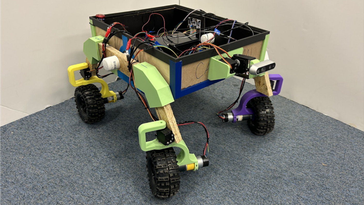
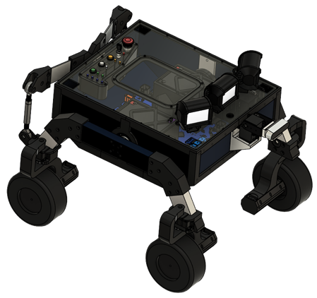
However, this rover lacked structural integrity, suspension, and maneuverability. This led to our final prototype, seen below:
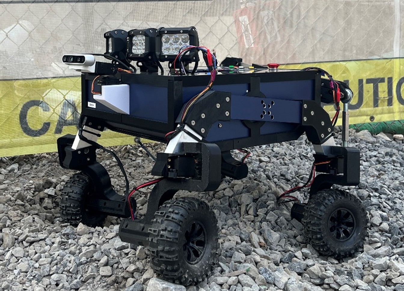
This final build provided many improvements from the V1 chassis, and enabled a more complete execution of our design intentions. The aluminum construction, paired with full implementation of the 4-wheel drive, 4-wheel steering, and rocker-style suspension, provides for optimal terrain handling. A custom PCB with an STM32 microcontroller, located inside the hull of the rover controls the driving and steering, as well as collects sensor data from the IMU and air quality sensors. The automotive-grade LED lighting mounted on the lid of the rover illuminates the cave for the Intel RealSense camera on a pan-tilt system to better visualize the cave environment. An Nvidia Jetson running ROS2 interprets that camera data, determines a path for autonomous navigation, and provides movement commands to the microcontroller. The system can also be driven manually by pairing a wireless controller to the Jetson. Upon completing traversal of the area, the images taken by the camera are then stitched together to create a human-viewable 3D map of the cave for safety assessment. Each of these subsystems will be further discussed in the sections following the system diagram.
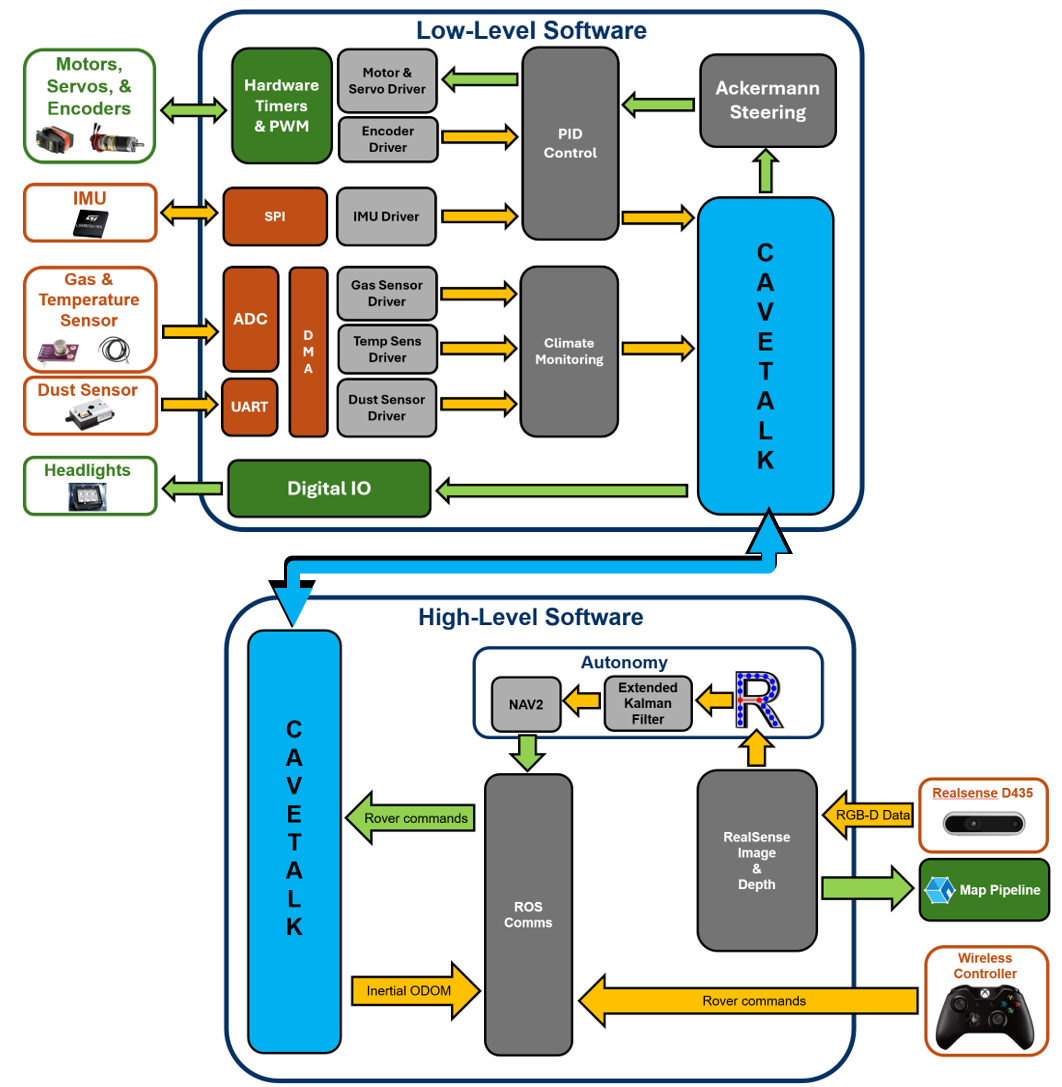
There are 4 main components to this system. First, there is the chassis and hardware. We have a custom circuit board called the CAVeBoard running the rover. This has a central microcontroller chip called the STM32, which takes in IMU and other sensor data, and outputs movement controls for the motor drivers, steering servos, and headlights. Additionally, we have implemented a 4-wheel drive and 4-wheel steering system with a rocker-style suspension inspired by the Mars rovers for optimal terrain handling.
Next, there is the low-level control software running on the STM32 microcontroller. This is the code that interfaces directly with the hardware, controlling the driving and steering, and interpreting sensor data. A kinematic model of the Double Ackermann steering system is used to convert trajectory data from the navigation module into wheel speeds and steering angles, and feedback control is applied to wheel speed using a PID controller. In addition to trajectory data received from the navigation module, readings from the IMU, encoders, and environmental sensors are sent back to the navigation module over our custom CAVeTalk protocol.
The high-level software of the navigation module consists of ROS running on an Nvidia Jetson development board. This is where the wireless controller connects for manual driving mode, sending movement and configuration commands. This also receives color and depth image inputs from the RealSense camera, which informs our autonomous driving mode.
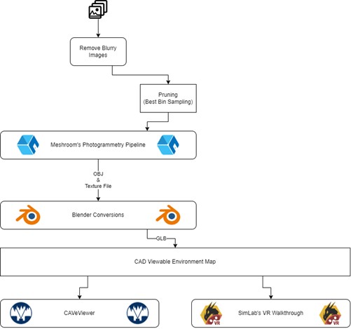
These images are then used in our fourth component, the map generation pipeline. In this process, we removed blurry images, prune down redundant photos, and sent them through a third-party software called Meshroom to create the 3D model. We combined the files in another third-party software named Blender to make it a single map file, which will output to our map visualization software.
Mechanical Design
For this system's use case, the mechanical implementation was a very necessary consideration and design field to ensure optimal operability in situ. This was inspired by the design of NASA's Perseverance rover for Mars, which faced the similar requirement of needing to traverse unknown, uneven terrain.
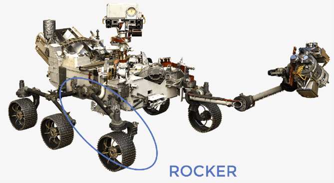
The main similarity between Perseverance and our rover lies in the suspension system. Perseverance uses a rocker-bogie suspension with a cross-body differential linkage which enables it to climb over large obstacles. CAVEMAN is much smaller in scale, leading to a scaled-down rocker suspension with a similar differential linkage, which provided similar agility. The full rover was designed in the Fusion 360 CAD software, as shown in the rendering below:
The rover was designed to be made of mostly 3D-printed or aluminum parts assembled with stainless steel fasteners from McMaster-Carr. Aluminum was chosen for its high strength-to-weight ratio and cost-effectiveness. The 3D-printed components were manufactured such that their infill patterns, density, and print orientation contributed to overall strength while minimizing material usage and weight.
Each wheel assembly contains a drive motor and steering servo, which provide for 4-wheel drive and 4-wheel steering capabilities. Paired with the aforementioned rocker suspension, these features enable the rover's offroad handling capabilities.
The central hull is where the PCB, Jetson, and batteries are securely mounted. These items are positioned so as to keep the center of mass located as close as possible to the 2-dimensional center of the rover itself. This aids in keeping the rover steady while traversing uneven terrain.
The RealSense camera and its corresponding pan-tilt servo linkage extends from the front of the rover. It is positioned such that it is far enough away from the body to maximize range of motion and field of view, while keeping it close enough that it does not face additional risk to damage in case of collision. The headlights mounted behind the camera provide additional lighting to deal with the inherent darkness of some caves, and are arrayed such that the entirety of the camera's view is illuminated.
All of these choices accumulate into an overall enhancement of the system's functionality specific to the intended use case of cave exploration.
Hardware Design
Below is a summary of the rover's hardware system. This system can be broken down into the subsystems of power, PCB, peripherals, and the Jetson.
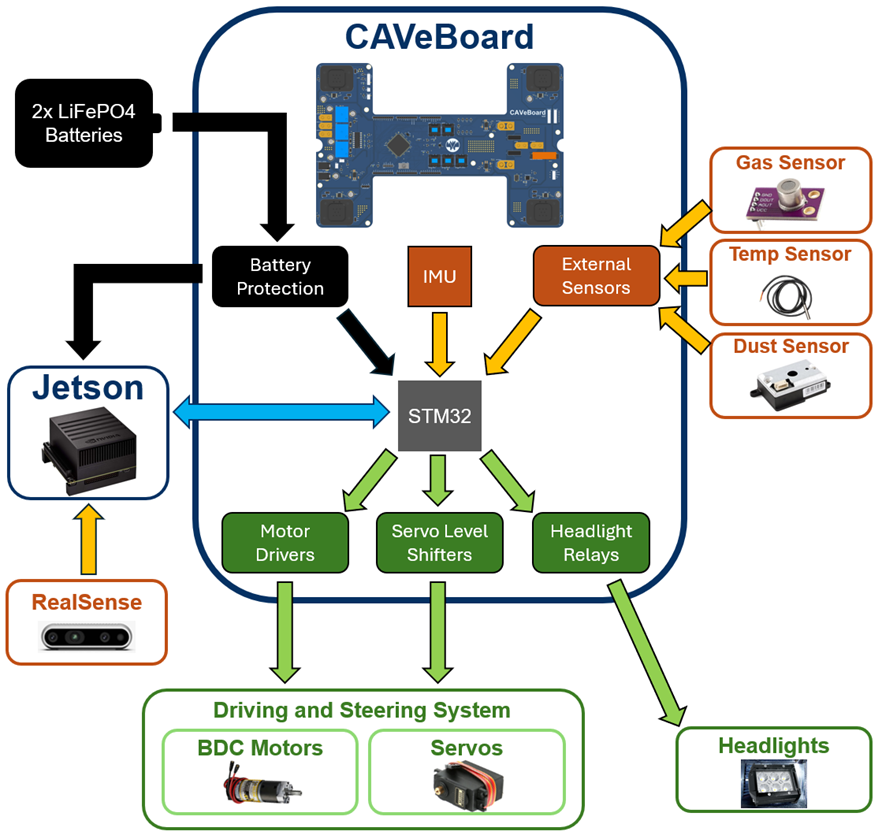
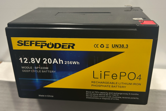
The rover is powered by 2 LiFePO4 batteries wired in parallel, each rated at 12V and 20Ah. Measurements taken upon receiving the batteries, however, indicate that at full charge, they are actually approximately 14V and 15Ah.
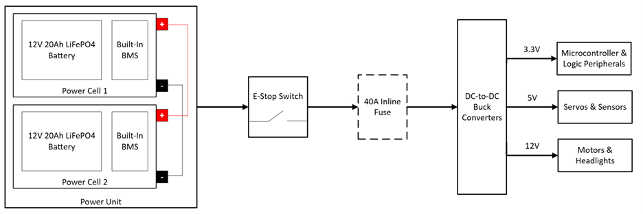
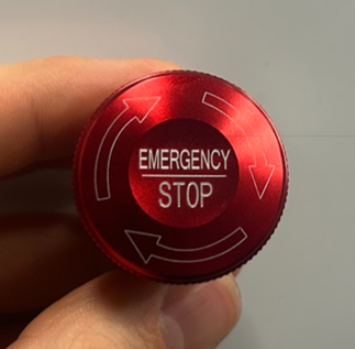
While these batteries come with a built-in BMS, we also implemented Schottky diodes and a 40A inline fuse for extra safety measures. The power flow from these batteries is controlled by an emergency stop switch, which then provides a 12V, 5V, and 3.3V line for the rest of the subsystems through various DC-to-DC buck converters.
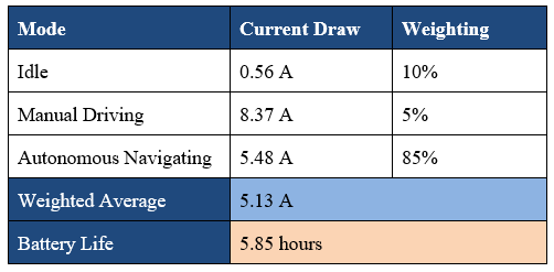
This system has significant power requirements from the various other components being supplied by these batteries, as well as some desired battery longevity requirements to meet. In order to calculate the battery life, current measurements were taken while the system was idling (on but not moving), operating in manual mode (holding maximum speed constant), and autonomous mode (reduced speed for camera-based obstacle avoidance). Those current draws could then be weighted based on how much of a power cycle the rover will likely spend in each mode. Based on these calculations, it is clear that the rover notably exceeds the desired minimum battery life of one hour.
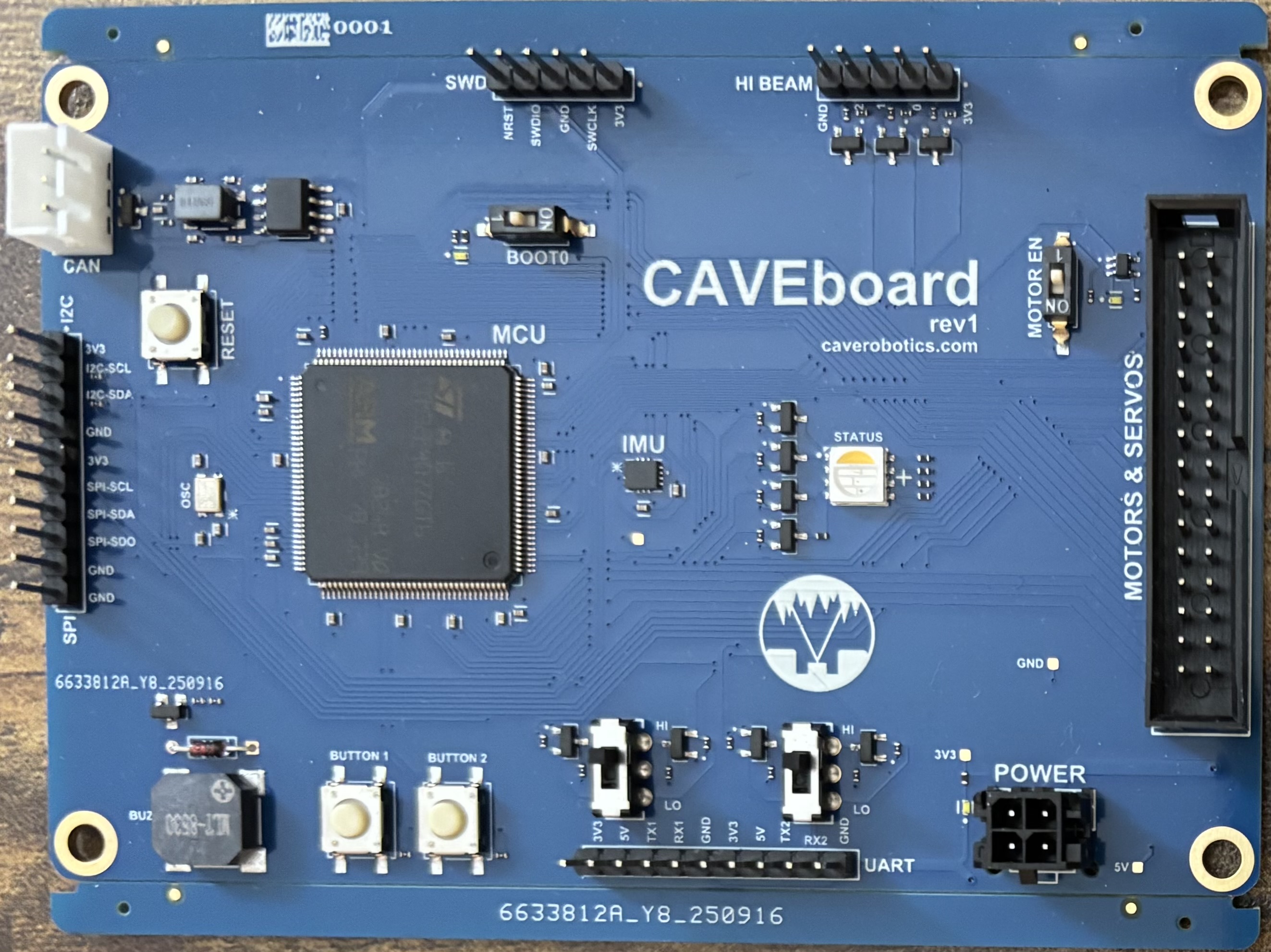
The next major component of the hardware system is the custom PCB, which has been named the CAVeBoard.
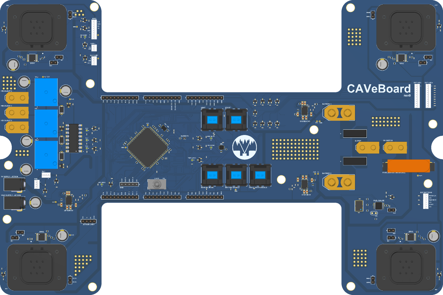
The batteries connect to the CAVeBoard through the XT90 connectors located on the right side of the board. The power flows through the diodes, e-stop, start switch, and orange 40A fuse to the buck converters, providing for the 3.3V and 5V rails.
The 3.3V rail primarily serves to power the STM32 microcontroller, which controls the system. The STM32F407ZGT6 was specifically chosen for this PCB because it provides capability for the many PWM channels, general I/O pins, and serial communication lines required to support the peripherals implemented.
Located in the dead center of the PCB is the inertial measurement unit (IMU). It was placed there specifically to be able to provide the STM32 with the most accurate position and acceleration data possible. Connections to other sensors were provided through JST connectors.
The headlights were controlled by a digital output from the STM32, which toggled the blue relays located on the left of the board. This circuitry also utilized an optoisolator chip to help prevent back-current propagation. The barrel jacks for providing power to the Jetson are located adjacent to the headlight circuitry. There were two jacks included in the design, one carrying 5V and one with the direct-from-battery 12V, as there were multiple different Jetsons considered for this project with different power requirements.
Each corner of the PCB has a DRV8874PWPR motor driver chip, which takes a PWM signal from the STM32 and shifts it up to 12V using an h-bridge to drive our motors, while limiting the current drawn by each motor to be about 5A.
The steering servos also necessitated logic level shifting on their PWM signals as they required 5V logic instead of the STM32's 3.3V PWM signal. This was achieved through the following bidirectional level-shifting circuit:
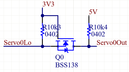
These motor, encoder, and servo lines all connect to their respective components through the Mil-Spec connectors located on each corner of the CAVeBoard. Given the significant current draw of all of these components, the original design included 1.98mF of parallel electrolytic decoupling capacitors dispersed across the board to maintain the 12V rail in case of current surges. However, that was eventually found to be insufficient during the stage of the motors beginning to drive, given that is the point of highest torque and consequently highest current draw as the motors overcome static friction. As such, the overall decoupling capacitance was increased to 9.0mF, which smoothed out the blips.
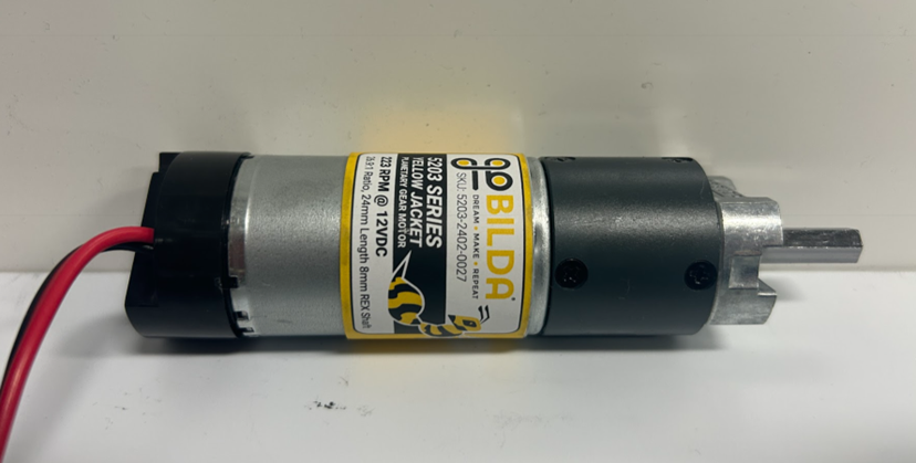
This leads into the third component of the hardware system: the peripherals. The most important hardware peripherals on CAVEMAN are its drive motors. These are 12V brushed DC motors sold by goBilda with a built-in 26.9:1 reduction gear box for increased torque. With a maximum speed of 223RPM and our wheel radius of 80mm, these motors could theoretically enable our rover to reach speeds of up to 1.87m/s or 4.18mph. However, our experimentally-determined top speed based on reading from the built-in encoders while the motors were fully loaded was closer to 1.5m/s or 3.36mph. This is still faster than is required for our system to traverse through caves.
The steering and camera pan/tilt movements were operated using standard 20kg MG995 servo motors with an operation range of 180 degrees. These had no issue performing the steering or camera movement commands, even while bearing the full weight of the system.
Additional outputs include our automotive-grade LED headlights rated at 1A and greater than 1200 lumens, dust sensor, gas sensor, and various indicator LEDs used to show the state of the system and indicate errors.
The final component of the hardware system is the Nvidia Jetson development kit and the Intel RealSense camera. The camera connected over USB to the Jetson to provide live camera data for navigation and stored RGBD data for post-traversal map generation. The Jetson communicated with the STM32 microcontroller using UART and our custom CAVeTalk protocol, which is discussed later. This UART connection was made with the help of a secondary custom PCB, called the CommET, short for Communication Expansion Tool.
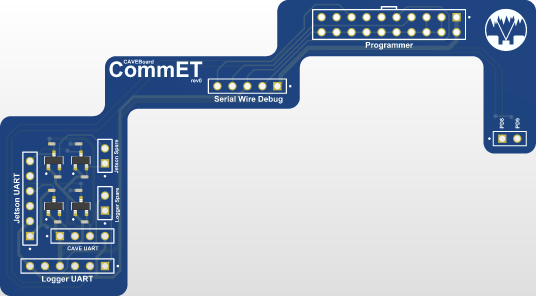
The CommET mounts directly on top of the pin headers on the CAVeBoard, similar to how Arduino Shields or Raspberry Pi HATs connect to their respective microcontroller developer boards. This addition level shifts the UART so that the STM32 can use 3.3V logic and the Jetson can receive 5V logic through a USB to UART adapter. This board also provides the capability to connect a second UART adapter to add a logger, as well as the 20-pin ST-Link V2 connector for programming the CAVeBoard via serial wire debug.
All of these various boards, power sources, peripherals, etc, come together to form a comprehensive hardware system that enables this rover to operate as intended.
Embedded Systems & Low Level Control
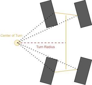
CAVEMAN utilizes a so-called Double Ackermann Steering System in which the front and rear pairs of wheels turn together. By steering with the front and rear wheels, the turning radius decreases by roughly half compared to the normal Ackermann Steering System found on most cars. Having a tight turning radius is important for maneuvering in confined environments underground. Additionally, because each wheel assembly can be individually controlled, steering can entirely be controlled in software by the Low-Level Control module. This eliminates the need for complex mechanical linkages and improves the mechanical reliability of the rover.
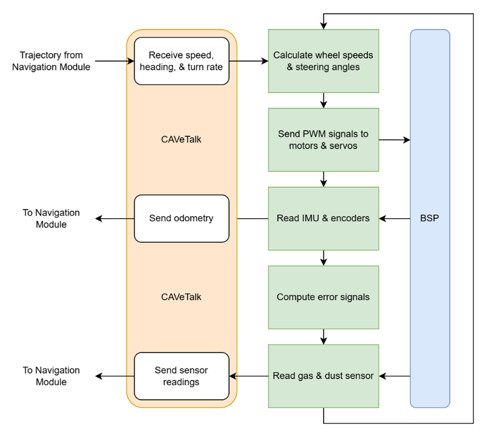
In addition to controlling a motor and servo for each of the four wheel assemblies, the Low-Level Control module is also responsible for controlling the pan and tilt servos for the camera, toggling the headlights, reading data from the environmental sensors, and communicating with the High-Level Control module. A diagram of the main peripherals the Low-Level Control module is responsible for and the interfaces with which they connect to the Low-Level Control module is shown below.
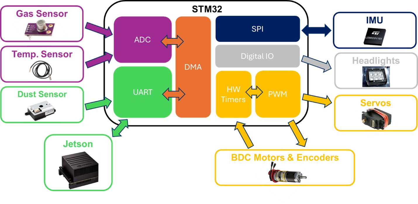
Based on the peripheral requirements, the STM32F407ZG was selected as the microcontroller to run the Low-Level Control firmware. It has enough hardware timers to support PWM for all of the motors and servos, all of the necessary communication interfaces for the sensors, and enough GPIO to physically connect all of the peripherals. The complete pinout for the microcontroller and peripherals can be found in the Appendix. With a clock speed of 168 MHz, it is also sufficiently fast to run the control algorithm loops at 1 kHz to 4 kHz while simultaneously maintaining the 1 Mbps communication link with the High-Level Control module.
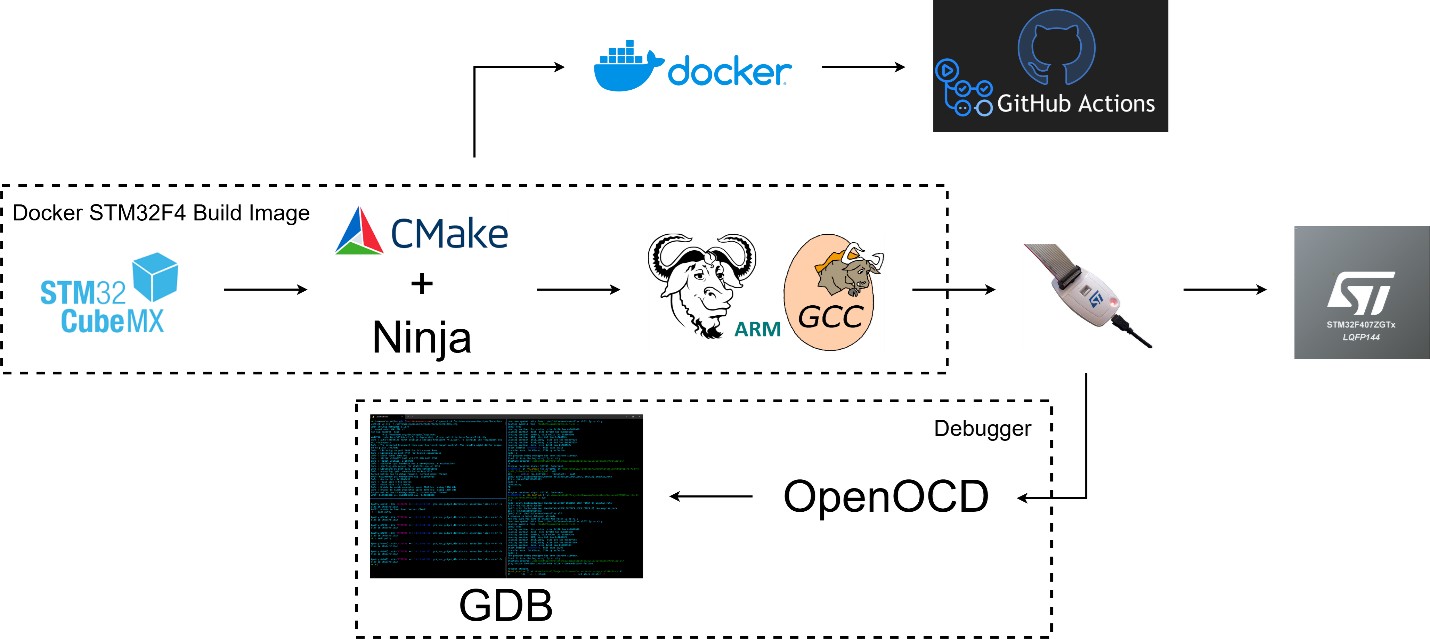
In order to program the STM32F407Z microcontroller, a custom Docker image with the necessary tooling was created. STM32CubeMX was used to do pin planning and generate ST's Hardware Abstraction Layer (HAL) for this particular microcontroller. The buildchain consists of CMake, Ninja, and GNU ARM toolchain. Together, OpenOCD and GDB were used to program and debug the microcontroller. GDB connected to OpenOCD which talked to the microcontroller via an ST-Link and Serial Wire Debug (SWD). The Docker image was also used to run Continuous Integration and Continuous Deployment (CI/CD) jobs on Github Actions. These CI/CD jobs include automated build checks, static analysis with Cppcheck, and formatting checks with Uncrustify. If all checks passed, a CI/CD job published an artifact with the latest build of the Low-Level Control module firmware.
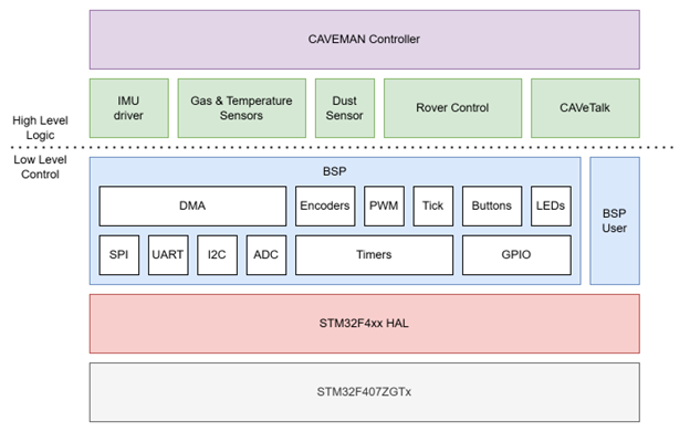
The Low-Level Control module software is arranged into layers to abstract the higher-level logic from the lower-level hardware control. The ST's startup code and HAL for the STM32F407ZG sit at the lowest layers. On top of that sits the custom Board Support Package (BSP) for CAVEMAN. The BSP provides a board-agnostic API for interfacing with hardware, allowing motor, servo, and sensor drivers, control algorithms, and communication stack to run on any board supported by the BSP without the need to re-write any of the high-level logic. This is primarily accomplished using a series of lookup tables to encapsulate individual differences in hardware between boards. These lookup tables, which are part of the “BSP User”, all fulfill a common interface, allowing the core of the BSP to remain largely unchanged between boards. Having a BSP was important because several different boards, including the Nucleo-64, STM32-E407, and CAVeBoard, were used for development and testing over the course of this project. Moreover, a layered approach to the overall software stack improves code organization based on functionality and proximity to hardware as well.
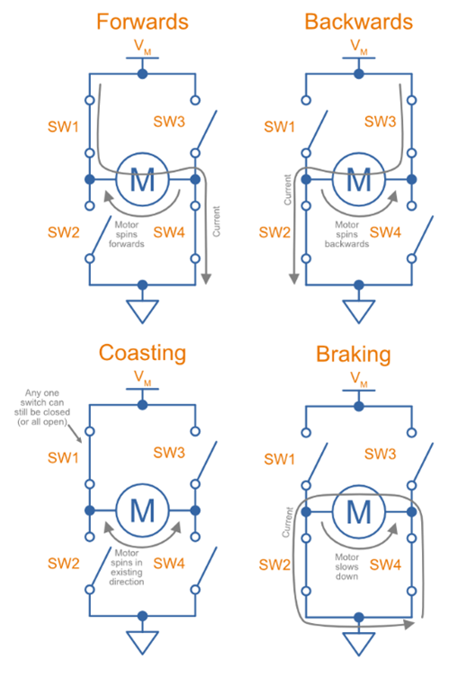
Custom drivers were written to control the motors and servos. Both motors and servos were driven using PWM signals generated by hardware timers. The motor driver used two sets of timers to individually control each of the two phases of each of the four brushed DC motors. This allowed each motor to be driven at different speeds and in different modes, including forwards, backwards, coasting, and braking.
An upcounting hardware timer was used to provide a monotonically increasing 1us tick since the encoder driver, IMU driver, and control algorithms required a clock with this level of precision. An interrupt is used to count timer overflows, and then the following formula was applied when sampling to get the tick where ARR is the value of the timer's auto-reload register and CNT current value of the timer's count register.
Tick = (Overflows * ARR) + CNT
In order to prevent a race condition if the interrupt occurred while sampling the tick, a Boolean flag was used as a pseudo-mutex to achieve synchronization. This works because Booleans are stored as 8-bit integers and read/write operations on integer types up to and including 32-bit integers are atomic on 32-bit ARM processors. A similar technique to prevent race conditions when sampling encoder data was applied to the interrupt that handles counter overflows for the hardware timers counting encoder pulses.
Each motor has a built-in encoder with two phases. The pulses from one phase will slightly lead the pulses from the other phase depending on the direction the encoder is rotated.
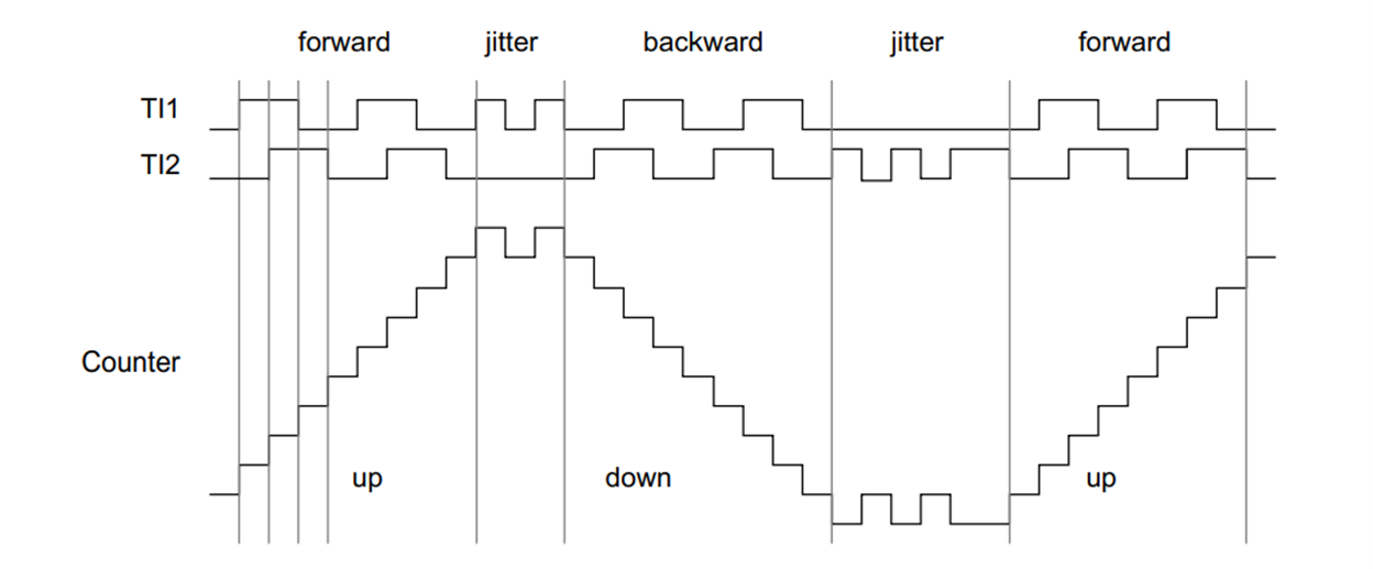
This allows the encoder driver to determine the angular position of each wheel which can be differentiated to find angular velocity. Hardware timers were again used to count the number of pulses from the encoders and determine the direction of rotation. These values were sampled in software to calculate angular position and velocity. An exponential moving average (EMA) was applied to results of these calculations to smooth out any jitter in the measurements.
s' = ax + (1-a)s
s += a(x-s)
a = smoothing factor, x = sample, s = smoothed sample
Angular position and velocity calculated from the encoders are used for wheel speed feedback control and for odometry in the High-Level Control module.
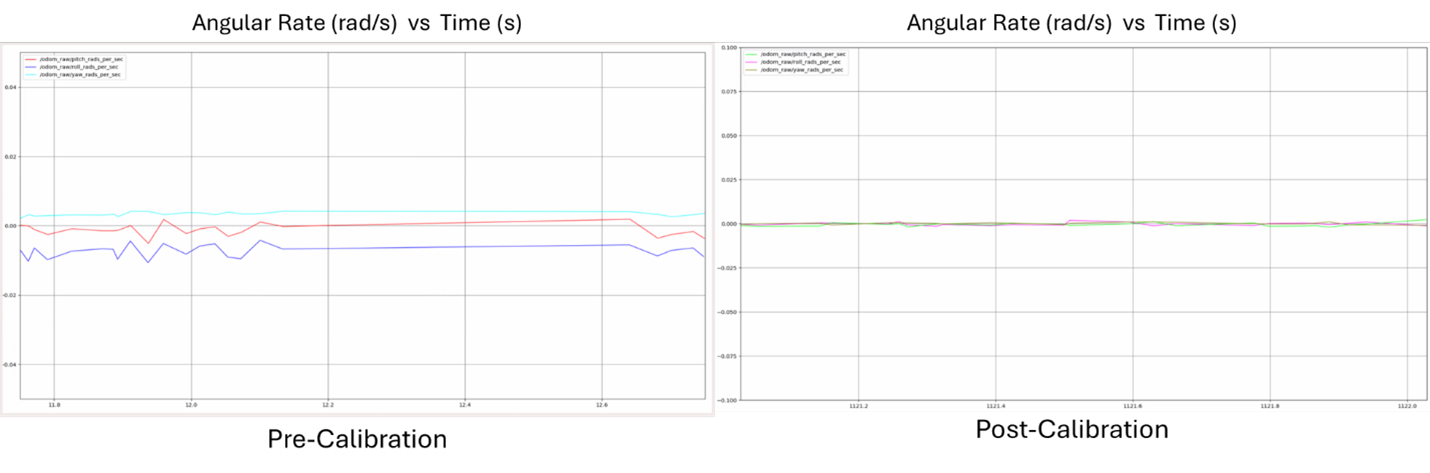
The LSM6DSV16X was used to provide linear acceleration and angular rates. The driver from ST, the makers of this IMU, was used to configure the IMU to apply low-pass filtering in hardware and automatically fuse accelerometer and gyroscope data into a pose estimated that could be read as a quaternion. Communication with the IMU is performed over SPI. On top of this driver from ST, a custom self-calibration procedure was written to remove any bias in the sensors. This involved slowing the sample rate to fill an onboard FIFO over the course of 1~2s with only accelerometer and gyroscope readings while the rover is at rest, then averaging the readings while taking into account the expected effects from gravity to calculate a bias which could be removed from any future readings after restoring the sample rate. Data from the IMU is used for odometry and pose estimation in the High-Level Control module.
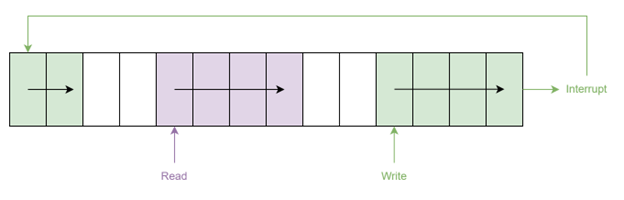
The Low-Level Control module uses three UARTs: one to communicate with the High-Level Control module, one for logging, and one for reading data from the dust sensor. All three UARTs use DMA and ring buffers to send and receive data. The Low-Level Control module communicates with the High-Level Control module using the CAVeTalk protocol over UART. The logging UART directly outputs log messages as ASCII text.
A custom driver was written to read data from the DC01 dust sensor over UART according to the following protocol. The data returned from this sensor is the total level in ug/m3 of PM2.5 and PM10 size particles in the air. Data from the dust sensor is used to determine if the level of particulates in an environment is safe for humans.
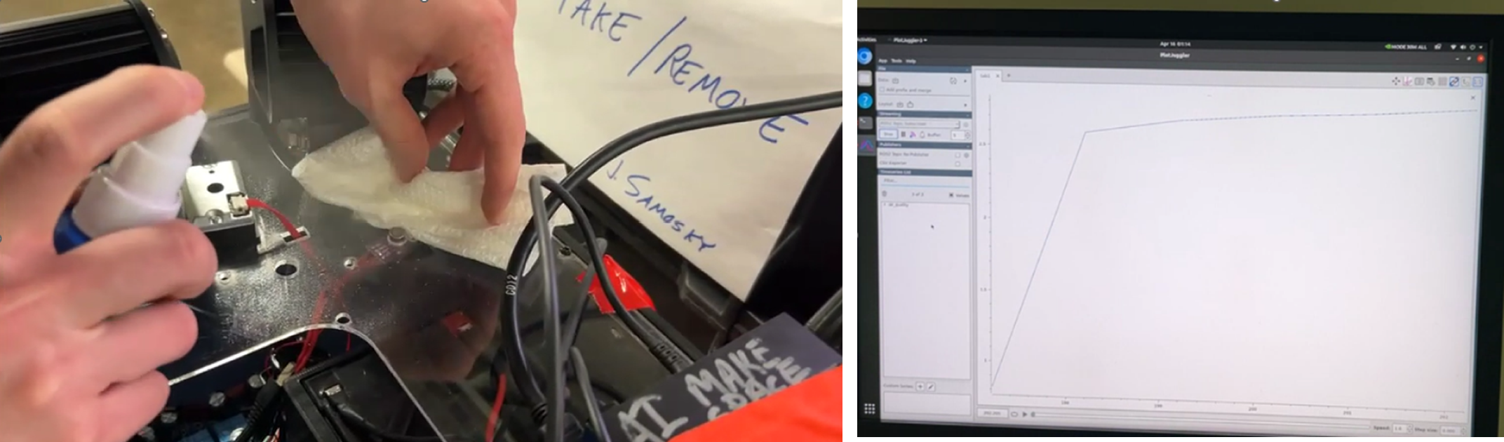
An ADC was used to read data from the onboard temperature sensor and gas sensor. DMA was also used to read the data from the ADC. The gas sensor produces a variable voltage in response to the level of volatile organic compounds (VOC) present in the air. Some examples of VOCs include formaldehyde, toluene, and organic solvents. These and many other VOCs are often used in mining applications and some such as methane can occur naturally underground. Depending on what specific VOC is being measured, the variable voltage readings from the gas sensor are fitted to different curves. Therefore, only the raw voltage readings are logged and different curves can be fit to the data after-the-fact depending on the target VOC. Some example curves are shown below.
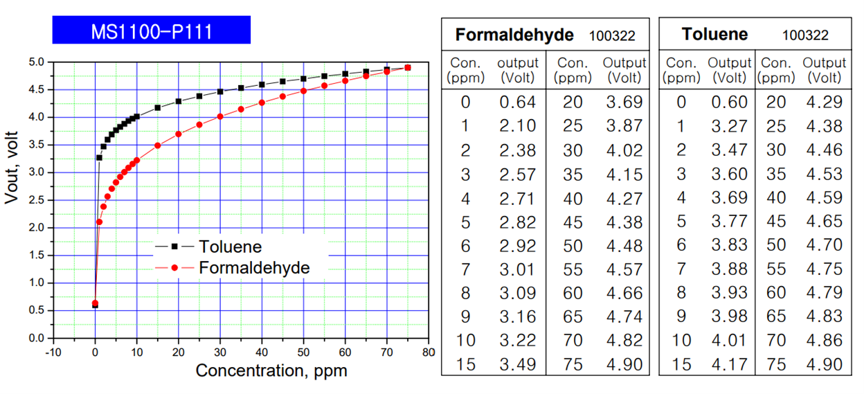
Data from these sensors are used to determine if the temperature and level of VOCs in an environment are safe for humans.
LEDs are controlled by digital outputs and buttons are connected to digital inputs. The LEDs are used to indicate various statuses, such as if the rover is armed and if communication between the Low-Level Control and High-Level Control module is healthy. The buttons allow a user to manually perform functions like arming/disarming and toggling the headlights, which are another digital output. The digital inputs for the buttons are read by interrupts and a configurable debounce is applied to each.
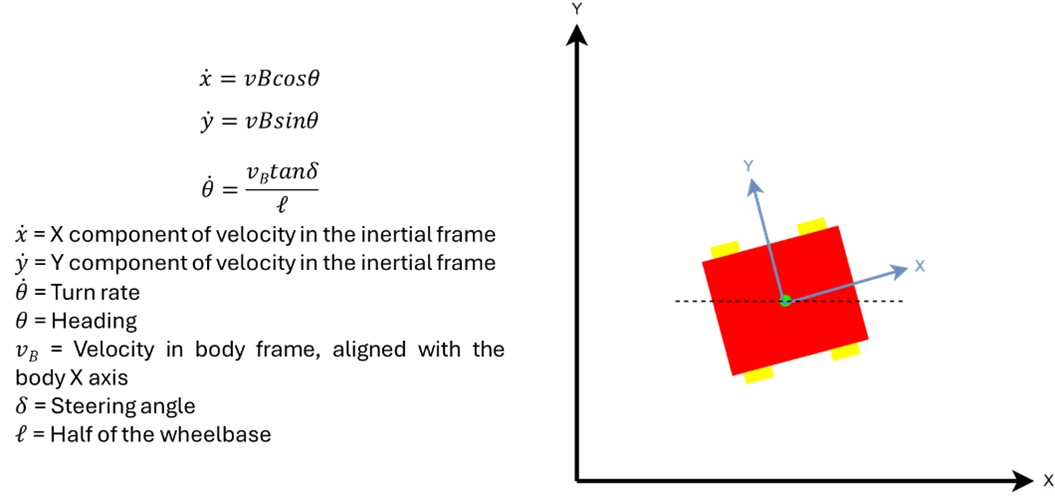
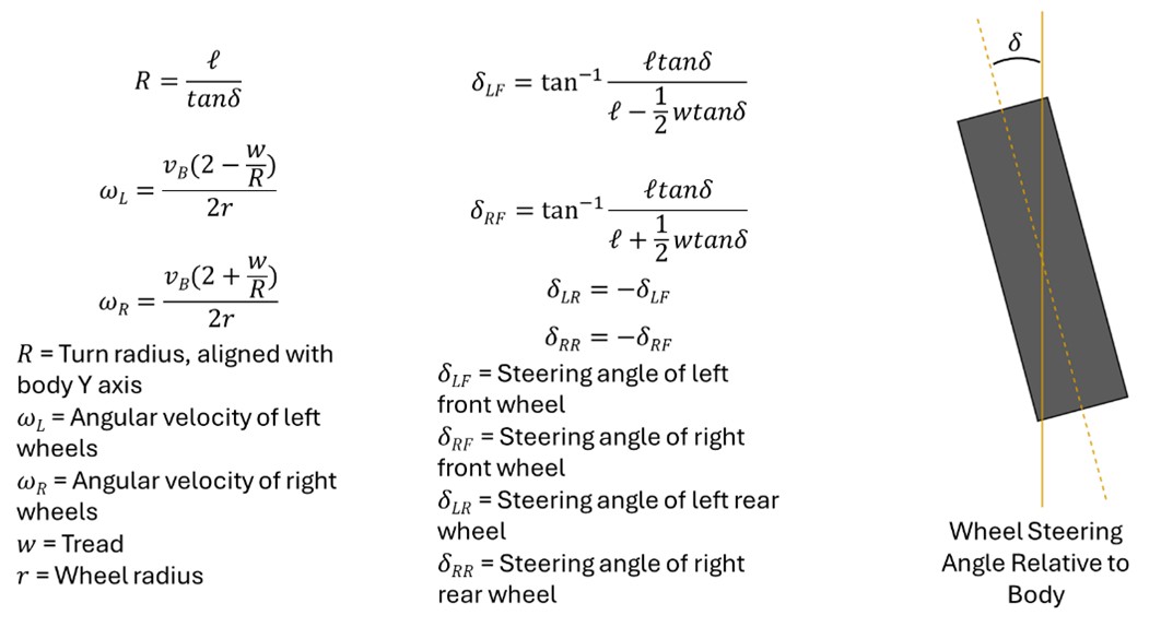
The following kinematic model of the Double Ackermann Steering System was developed to allow the Low-Level Control module to convert trajectory data received from the High-Level Control module into individual wheel speed and steering angles for each of the four wheel assemblies. The Low-Level Control module receives this trajectory data in the form of a linear and angular velocity.
The Low-Level Control module runs a main loop that performs the following tasks:
1. Receives trajectory data from the High-Level Control module over CAVeTalk if new data is available
2. Use the kinematic model of the Double Ackermann Steering System to update the commanded individual wheel speeds and steering angles
3. Read linear acceleration, angular velocity, and the pose estimate of the rover from the IMU and wheel speed from the encoders
4. Send IMU and encoder data to the High-Level Control module at a rate of 50~100 Hz
5. Apply PID control to the speed of each wheel using feedback from the encoders
6. Read gas, dust, and temperature levels and send the environmental data to the High-Level Control module for logging at a rate of ~1 Hz
While some tasks within the main loop run at lower frequencies, the entire main loop runs at a frequency of 2~4 kHz.
In addition to the tasks executed in the main loop, the Low-Level Control has functionality that allows it to be armed/disarmed and configured over CAVeTalk. Arming enables all motors and servos while disarming conversely disables all motors and servos. This is a safety feature to prevent accidental movement or runaway behavior, which is especially important when CAVEMAN is being controlled manually. When the rover is disarmed, various parameters like servo movement bounds, EMA smoothing factors, and PID gains. This is useful when testing and tuning the rover. Lastly, the Low-Level Control module has a logging feature that can be configured to log messages depending on their log level. This means more verbose logging can be enabled during testing and debugging but set to a less verbose level during normal operations to avoid polluting the logs with unnecessary information. The logging level can also be configured over CAVeTalk without needing to compile the Low-Level Control firmware.
To interface between our microcontroller and our Nvidia Jetson, we developed a UART-based communication protocol called CAVeTalk, short for Cave Autonomous Vehicle Talk. Using UART as our serial protocol, and Google's protocol buffer library to handle consistent serialization and deserialization of any data type, CAVeTalk serves as an extensible wrapper for easy interfacing between port-level bytes and controller-level actions.
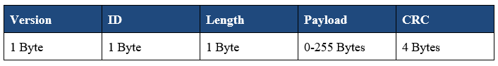
CAVeTalk consists of two levels, the link layer and the interface layer. The link layer is a C-based state machine that controls the sending and receiving of bytes, while also leaving the implementation abstracted so that it can be tailored to any machine. The state machine ensures that the packet reception is decoupled from reception time, looking at the actual data availability to determine if all the packet information is present. The basic packet structure is a header, payload, and cyclic redundancy check. The header consists of the version, ID, and length associated with the payload.
The interface layer allows the messages to be processed in both directions, for sending and receiving, also customized to different computer systems. For microcontrollers, there is a specific ANSI C-based version of Protocol Buffers called NanoPB, while the standard Protocol Buffers library is backed in C++, which was used on the Nvidia Jetson. The interface layer is directly responsible for serialization and deserialization, along with higher-level control interfacing. For receiving packets, the header and CRC are used to validate the payload and route it to the correct deserialization function, which then allows the information to be passed to a callback that interfaces with the control systems. For example, a Movement command, when received, is routed to a HandleMovement function where it is deserialized and then passed onto the callback where it would steer and spin the wheels. The opposite path is used for sending messages, where higher-level control sends a message with all its payload information, and then it is serialized accordingly, and pushed to the link layer where it is appropriately wrapped and sent over the wire.
CAVeTalk uses CMake and Ninja as our foundational build system for code compilation, building, and running tests. Cppcheck is used for static analysis, while Uncrustify is used for code formatting. The GoogleTest library is used for unit testing each part of the communication protocol. Unit tests rely on a ring buffer implementation to simulate UART hardware port buffers. The common layer is tested specifically for sending and receiving errors, along with individual parts of the message byte structure. The interface layer is tested for data integrity through serialization and deserialization, ensuring that packet lengths are within the 255-byte limits and that data values are preserved regardless of type and precision. Custom object assertions were written to ensure that the unit-tests could thoroughly test message data in an automated manner. Gcovr was used to generate code coverage reports to ensure that unit testing was thorough and complete to the best of our ability, and code coverage for the link layer is at 95% while the C interface layer sits at 89% and the C++ interface layer is at 93.5% code coverage. Github CI/CD was used to ensure each commit and pull request was consistently tested and formatted automatically, before branches were merged into main.
High Level Software & Robotics
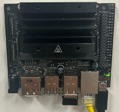
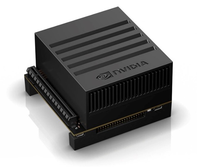
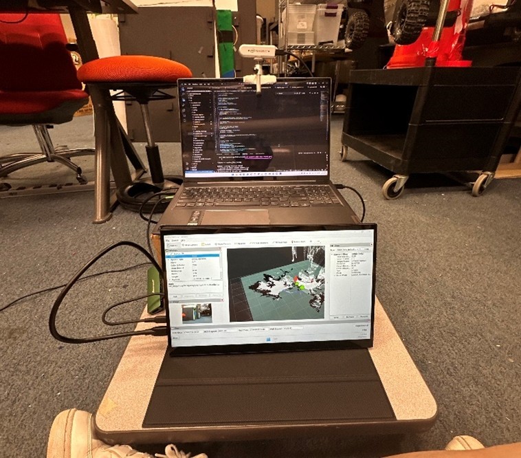
The high-level software exists on our “Navigation Module”, which is an Nvidia Jetson device. Various factors went into our selection of the Nvidia Jetson family, but compute power is the primary reason. The Jetson devices provide on-board dedicated GPUs that harness the power of Nvidia's CUDA framework for parallelizing and accelerating graphical, computer-vision, and machine-learning tasks that are critical to the performance of our system. Packages such as OpenCV and TensorRT can be built with CUDA support such that the accelerated processing propagates throughout higher-level packages that depend on them. We started our exploration of the ecosystem, setup of our software development-workflow, and development of lower-level communications and controls on a budget-friendly Jetson Nano Developer Kit.
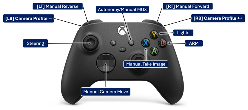
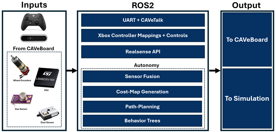
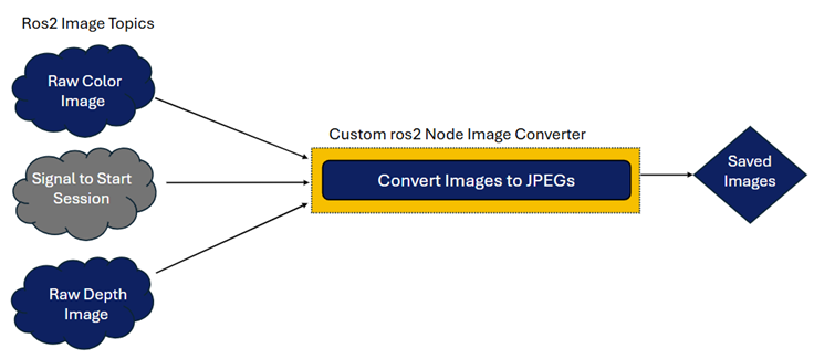
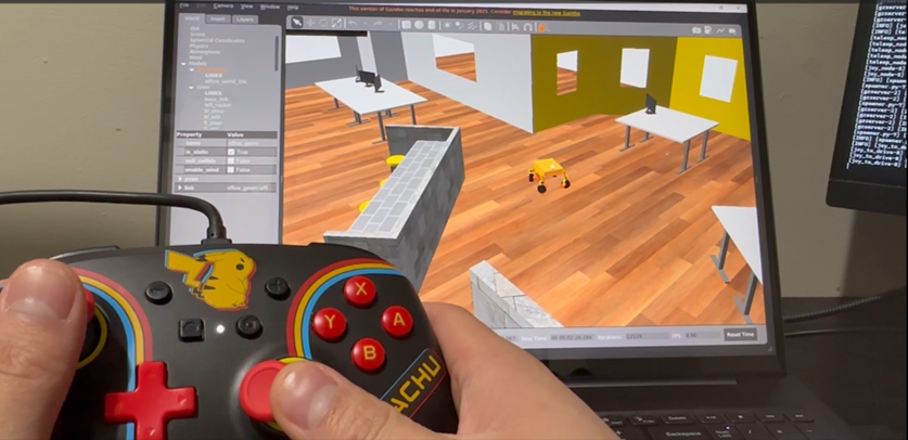
With foresight of future device and platform changes, we used Docker for consistency, portability, and scalability of our software between multiple devices: ARM64 with Ubuntu18, AMD64 with Ubuntu22, and finally, ARM64 with Ubuntu20. Within the containers, we used Robot Operating System 2 (ROS2), a software framework for robot development frequently used in robotics research. The ROS2 framework provides modularity and scalability through its distributed graph architecture for internode communication, where nodes can be written to subscribe and publish to topics dynamically. We utilized the modularity of the ROS2 framework to facilitate parallel development of our custom packages for the following functionalities: UART + CAVeTalk protocols, Xbox Controller mappings + controls, RealSense Camera APIs + controls, and Autonomy + Navigation. The UART + CAVeTalk protocols package consisted of the low-level UART communications, CAVeTalk, and configuration settings that were used to facilitate parameter tuning and testing with the CAVeBoard in lower-level tasks such as motor and PID tuning. The Xbox Controller mappings + controls package reads from a Bluetooth Xbox Controller - which serves as our primary user-interface - to control the rover, the full controller functionalities can be seen below. The RealSense Camera APIs + controls package interfaces with the open-source ROS2 RealSense package to customize camera capture quality, framerates, and post-capture conversion of raw image data to JPEG compressed images, a diagram of this is depicted below. The Autonomy + Navigation package consists of sensor-fusion, cost-map generation, path-planning, and behavior-trees. A broad summary of this software structure is depicted below. Also shown is an output to simulation, which was made in Gazebo Classic to simulate depth cameras, IMUs, and wheel-encoders - as well as to have an early test of control kinematics. This simulated environment's main purpose was to develop autonomy before a physical test rover prototype was available and it was dropped by the fabrication of our first rover prototype.
Due to the computationally intensive workload of our automation and navigation stack, we migrated our development over to a higher-power Jetson Xavier AGX. The Autonomy + Navigation package utilizes an Extended Kalman Filter to combine Visual Odometry generated by RTABMAP using RealSense Camera data, with wheel encoder and imu data for a robust fused odometry for localization within a map. This fused odometry along with a cost-map generated from RTABMAP can be used by NAV2 (which provides the obstacle avoidance capabilities), along with a target destination, to process, plan, and send drive commands according to a customized behavior tree. Our NAV2 configuration utilizes an A* pathfinding algorithm to choose a path, combined with a “Regulated Pure Pursuit Controller” (RPPC), which computes a regulated non-linear steer curvature and path to a selected destination. Our behavior tree additionally defines recovery behaviors in case a collision is detected, or if the rover is stuck: to wait, then back-up. Finally, we utilized the Depth-First Search (DFS) algorithm to guide exploration and set destinations as inputs into NAV2, which then outputs drive commands out to the CAVeBoard.
Included in the high-level software were the configurations of the low-level rover parameters. These configurations were integrated into the communications library of the rover, allowing the specific ROS comms package to handle the sending of configurations before starting the rest of the communications program. These configurations were written in XML so that they were both machine- and human-readable and could be changed without having to rebuild entire programs or packages. They were parsed using tinyXML2 at the start of the program. There was a CAVeTalk-specific file that handled physical parameters that were outlined in the CAVeTalk configuration messages, all listed above. This controlled things like the camera servo bounds, the wheel servo bounds, the motor operating parameters, the encoder operating parameters, the microcontroller log verbosity, and PID parameters for the wheel speed and turn rate. The next configuration file was for the custom camera movements, which allowed any number of profiles to be parsed and linked to a specific index, such that it can be changed by a controller or by other code segments. The profiles contain any number of movements with specific durations attached, and they automatically loop back to the first movement. This simple model allows any number of movements and profiles to be made, accessed, and played on the rover for an optimal mapping experience. The final configuration file uses a constantly reloading XML file to sending movements to the rover, either constantly looping or just sending a single time, and this was developed for PID tuning. The mechanism of control at the point of PID tuning was through a controller, which was user-friendly but not precise for tuning. This sender program augmented this control scheme, and with one additional configuration, the settings for control could be switched between manual mode, this CAVeTalk Sender program, and autonomous mode.
Mapping Pipeline
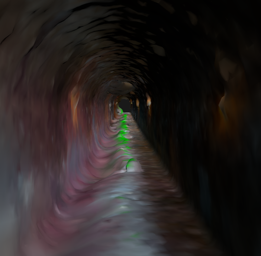
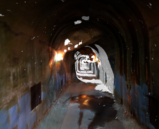
The mapping pipeline consists of taking the images captured by the ROS2 Realsense Node and converting those into a CAD-viewable map. The foundation of this system lies in a 3rd party software called Meshroom, that uses a technique called Photogrammetry to turn these images into a 3D model. Meshroom uses a node model to sequentially process and create the 3D model, starting with creating point clouds, then depth maps, then a mesh, and finally texturing the mesh. From there, these textured meshes resembled the explore environment, and can be viewed in a variety of manners including online or desktop CAD tools, along with virtual reality toolsets.
The images, once they were offboarded from the rover, needed to be pre-processed before going into the Meshroom photogrammetry pipeline. The basic steps were getting rid of the blurry images and then pruning the dataset without loss of integrity and information. Since the camera captured standard RGB and depth images at around 23fps, a 40 minute session yields over 55,000 RGB and depth images each. But many of them are blurry due to rover and camera movements, so they must be filtered out. Convolving each image with a Laplacian kernel converts the images into its 2nd spatial derivative, and then in that image, regions of fast change are highlighted. Taking the variance of the image as a whole gets the distribution of the 2nd derivative across the entire original image, and below a threshold of 150, the image is relatively blurry. This is not a definitive metric, but it closely models blur behavior, so it was used as a thresholding measure for removing blurry images.
A few different pruning methods were used to delete duplicate images. The first two algorithms tried perceptual hashing as a means to find visually similar images. The standard pHash (perceptual hash) and CRPH (crop-resistant perceptual hash) techniques were used to convert the images into hashes that could be compared against each other for both identical and similar matches. The difference between pHash and CRPH is that CRPH used a segmentation technique called watershedding to separate the image into distinct parts, hash those distinct regions, and create an array of hashes associated with each image. The comparison between pHash and CRPH was that while CRPH's ability to find duplicates was marginally better, because it accounted for the movement of the rover to create cropping in the images that would then be caught by the algorithm, the computation time of this hash was enormous when scaled up to 10s of thousands of images. The time difference between computation was maybe 3-5x longer than normal pHash, however even pHash's pruning ability was not amazing. Visually identical images would often be classified as different, meaning I still had many duplicates in the resulting dataset, which would increase the photogrammetry computation time and distort the results. We developed a custom pruning technique, deemed best bin sampling, to offset computation times and handle the dataset duplicates in a better way. Best bin sampling relies on the sequential nature of the camera captures to get the highest quality capture of a specific region and ensure that the next captured photo would be different enough for proper photogrammetry processing. Iterating through the images, a tunable number of images are put into a bin, usually around 10, and then the least blurry image in the bin is chosen to go into the final dataset. The bin collection is stopped prematurely when an image is vastly different from the previous one, ensuring that the bin only picks the best out of similar images. As such, the dataset can be reduced by 50-90%, vastly reducing computation time, all the while the dataset integrity is maintained and optimized for photogrammetry. This pruning method has resulted in our best, most comprehensive and detailed maps.
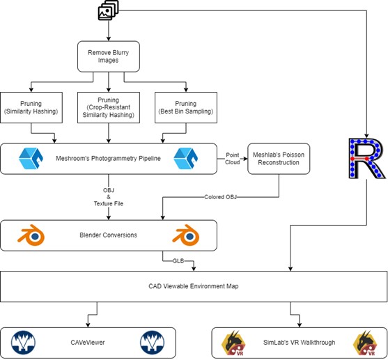
The 3rd party software, Meshroom, used a technique called photogrammetry to recreate a 3D model from 2D images in a modular pipeline system. This allowed us to customize the pipeline sequence and turn a lot of tuning knobs in the pipeline for testing. The photogrammetry pipeline consisted of using the images to stitch together features, create a point cloud, create depth maps, use these previous inputs to make a mesh, and finally texture that mesh. Under optimal circumstances, very little data was lost, but usually some exploration data was lost as the software considered the features or data to not integrate correctly into the entire map. An important thing to mention is that while depth data was collected, it was not used as a direct input for the photogrammetry pipeline. Development of a custom node utilizing the pre-existing depth data was attempted. While it was theoretically working, computation time was not decreased, and map accuracy was not improved, so it was not pursued further. The standard photogrammetry pipeline was used, though for automation, the command line interface was utilized in a series of PowerShell scripts.
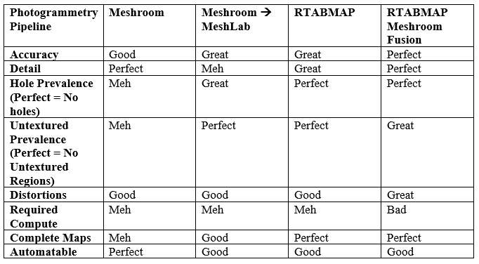
Additional mapping techniques leverages two other programs, RTABMAP and Meshlab. RTABMAP on the autonomy side had been tested to use the point cloud map that it generates from RGB and depth images to then reconstruct a surface from it using poisson reconstruction. The output was highly detailed but there was some residual noise from the movements and the live point cloud construction techniques it used. The artifacts in that reconstruction could be removed if the pictures were exported out of RTABMAP and put into the photogrammetry pipeline, ensuring a clean and proportional map of the explored area, though this sequence of events was infeasible on the autonomy compute modules and only tested on off-board devices. Similarly, poisson reconstruction could be used on the node that outputted a point cloud in Meshroom. Putting the Meshroom point cloud into a program called Meshlab, and running poisson reconstruction on it created a 3D map that, while slightly less detailed and a bit lumpier, were consistent in terms of output maps. Sometimes maps from photogrammetry would not give a complete map but a partial map of the explored area, and with inspection that data would be lost in the meshing stage. Using the raw point cloud and doing reconstruction from that ensured the map used the entirety of the data, though it still was not perfect. In the end, Meshroom's photogrammetry pipeline worked best for us.
The last step before viewing was using Blender from the command line to combine the output files into a single GLTF file. This file format is compatible with many other programs, like Powerpoint, WebGL, Blender, and other model viewers. The main benefit is having a single file to use for the map instead of an OBJ file, an MTL file, and an EXR file, plus other combinations for other methods. This unifying step ran quickly so its development was very smooth.
Viewing software for these maps comprised of pre-made, custom, and hybrid solutions. A standard viewer for validation and viewing for our team was 3dviewer.net, which allowed a quick check of the photogrammetry output. For user viewing, we derived two solutions of varying immersion. Our team created a custom GLTF web viewer, named CAVeViewer, where it uses Don McCurdy's three-gltf-viewer as a base viewer with added three.js logic on top for a tailored, playable map-viewing experience. This website is used to view all of the maps to ensure that all trials with outputs can be viewed for transparency and posterity. In addition to this viewer, we utilized SimLab VR to load GLTF files into a virtual reality landscape, adjust the scaling and placement of the model, and set the start point at the right position. This premade virtual reality viewer is limited in that in-game movement can only occur with point-to-point teleportation using the controllers or proportional real life movement tracking. The optimal traversal method would be joystick movement translated to in-game movement, but that option does not exist within this program. Both the CAVeViewer and the VR walkthrough videos are available on the caverobotics.com/maps/ website.
Testing
The motors were tested using a Nucleo-64 board and a breadboarded circuit using the intended DRV8874PWPR motor driver chips. The procedure for testing for the motors included sending PWM signals of various duty cycles to confirm the capability of turning at different speeds.
The servo motors were tested similarly, using a Nucleo-64 board and breadboarded level shifter circuit to send various 5V PWM signals at 50 Hz to confirm that they are able to turn the rover left and right along different angles.
Both of those tests were performed prior to design and ordering of our CAVeBoard PCBs to ensure that the circuit set-up worked ahead of time. These tests proved successful, with the motors spinning at the intended rates and reporting near the rated speeds, as well as the servos turning as required per their specifications.
The motors purchased also included built-in encoders. The first tests to ensure encoder functionality consisted of connecting them to an oscilloscope and visually observing the pules from each phase as the wheel was manually rotated.
Upon receiving the PCBs, they were tested by themselves before integrating with other system components. The first test performed was a thorough point-to-point continuity check. This was performed manually using a multimeter, specifically targeting power rails, the ground plane, and signal lines for the motor drivers, servos, headlights, IMU, and other sensors. The designed-in test-points were also validated with continuity at this time.

Once this was proven successful, the next step was to solder on the battery connectors, fuse holder, and other components for the battery protection circuitry. Then, once the battery was connected, a full-board power test could be performed. This consisted of verifying that all of the 12V test points were measuring in at the same voltage as the battery, as well as confirming the buck converters were functioning by checking all of the 3.3V and 5V rail test points. This test also proved successful, with both rails measuring within ~3% of their intended voltages.
The next test was to attempt to program the board and verify digital outputs. This involved connecting to the designated serial wire debug pins on the PCB with the ST-Link V2, toggling the boot switch to the correct position, and successfully programming the PCB to turn an LED on. This test was also successful.
Further PCB testing occurred in conjunction with the low-level control module, and can be found in the later integration section.
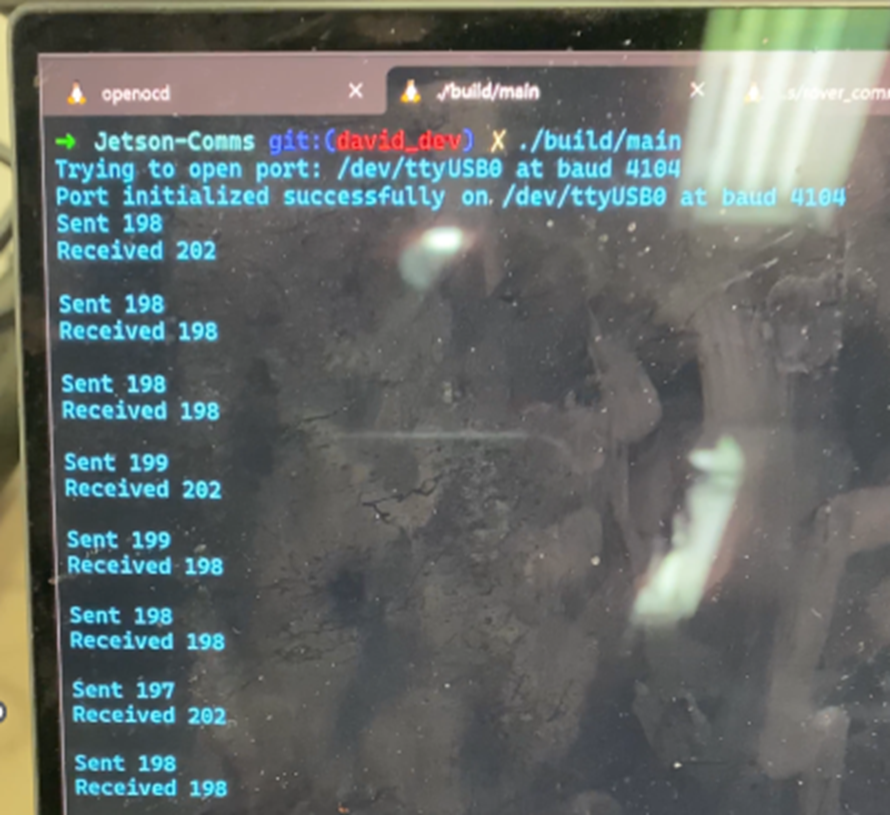
The UARTs were first testing by printing log messages to a serial terminal. Next, bi-directional communication was tested by using a TTL serial adapter to send a CAVeTalk “Ooga Booga” message from a PC to ping the Low-Level Control module and listen for a response. To confirm this, the Low-Level Control module logged when it heard a message and when it replied to it. The reply was then also observed on sending PC. For all of these tests, the baud rate was set to 1 Mbps since that was the maximum speed the TTL serial adapter was rated for. After confirming bi-directional communication worked, the maximum CAVeTalk message rate was tested. This was done by incrementally increasing the rate at which test messages were sent from the PC by 50 Hz. Each time the Low-Level Control module received a message, it would reply with another, meaning it was send and receiving messages at whatever rate the PC was sending at. To simulate real-world conditions, the messages being sent by the PC were primarily movement commands and the messages sent by the Low-Level Control module were primarily odometry messages. These tests showed that messages could be reliably transmitted simultaneously to and from the Low-Level Control module at a rate of 500 Hz. Beyond 500 Hz, errors would begin occurring within the first few seconds of transmission. However, a much lower message rate of 100~200 Hz was used in practice. Lastly, the effect of DMA was quantified. UART transmissions were timed in two ways: recording the microsecond tick at the start and end of a transmission to find the elapsed time and toggling a GPIO line at the start and end of a transmission and using a scope to measure the time between the rising and falling edges. Both methods revealed that the microcontroller required 3 ms to execute a UART transmission for the Ooga Booga message without DMA, and only 5 s to execute the same UART transmission with DMA. This means UART transmissions with DMA were roughly 600 times faster than UART transmissions without DMA.
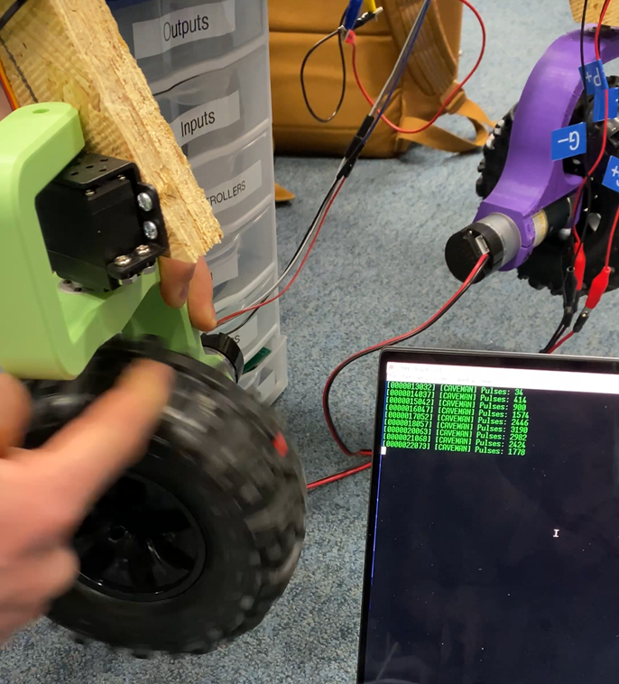
The encoder driver was tested first by spinning a wheel by hand and logging the position of the wheel. It was confirmed +4 rad was logged when the wheel was spun forward roughly two revolutions, 0 rad when it was spun back two revolutions, -4 rad when spun back another two revolutions, and +2 rad when spun forward three revolutions. To confirm the calculated angular velocity was correct, a piece of tape was placed on a wheel and the motor was spun at a constant 50% duty cycle. The wheel was elevated off the ground to avoid placing any variable load on the motor. The wheel was filmed in slow motion so that the number of revolutions could be determined by counting how many times the tape marking passed a specific point in the rotation of the wheel. The angular velocity was calculated by dividing the number of revolutions by the duration of the video. It was compared against the value logged from the encoder driver. The smoothing factor for the EMA applied to the encoder data was adjusted until the two measurements were consistent to within 0.25 rad/s one another. This process was repeated for each of the four wheels.
After the encoder drivers were producing accurate readings, they could be used to test motor speed. The motor driver was commanded produce PWM signals to spin the wheels forwards and backwards at 5 rad/s, 10 rad/s, 15 rad/s, and 20 rad/s. At each angular speed, readings from the encoders were compared to the commanded speed. Each motor was within +/- 1 rad/s for each commanded speed, which was deemed acceptable given that PID tuning would be applied to wheel speed later.
The servo driver was validated by commanding each servo to angles of 0.17 rad, /2 rad, and 2.97 rad and measuring the true angle with a protractor. If the measured angle was off by more than 0.01 rad from the commanded value, the bounds of the range of the duty cycle for the PWM signal were adjusted in software until the measured value was within 0.01 rad of the commanded value.
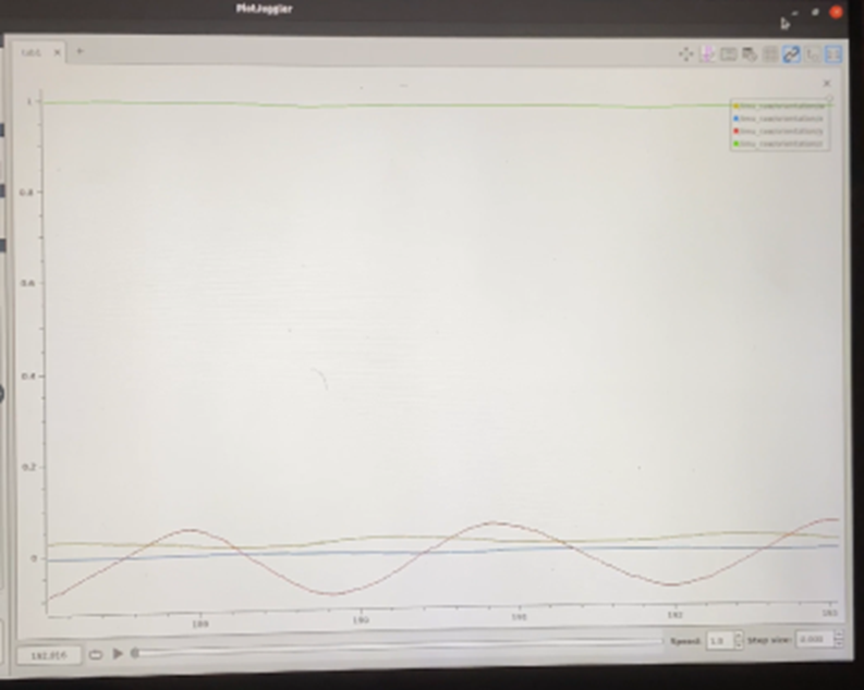
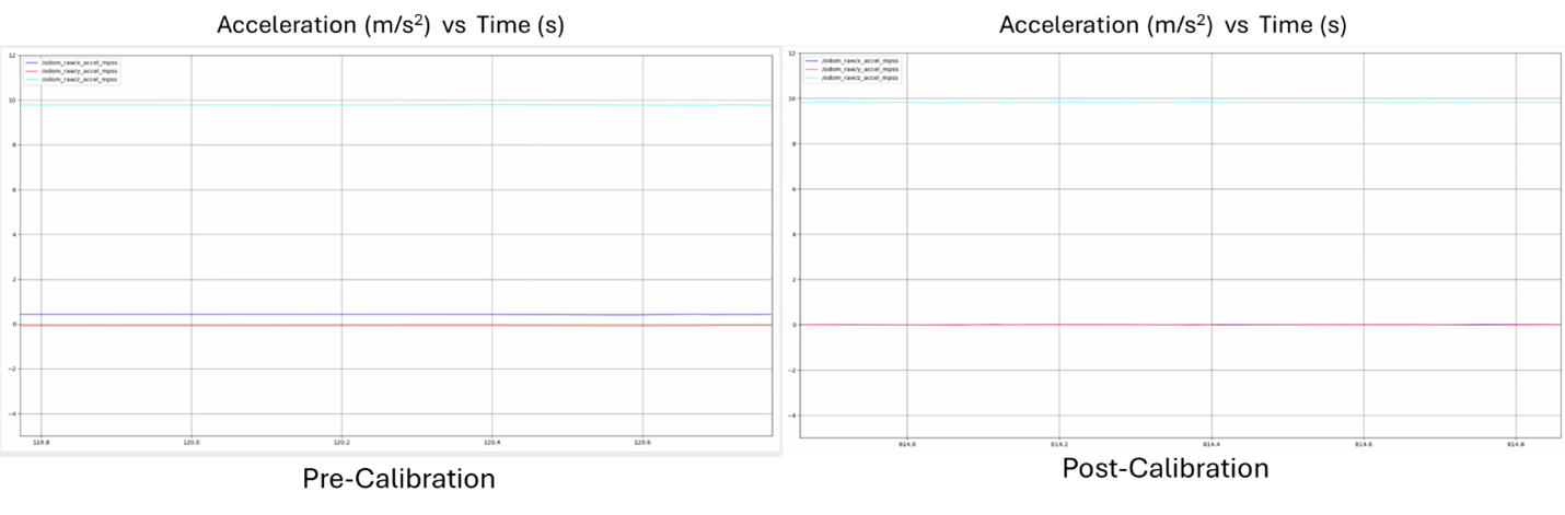
Since the Low-Level Control module sends data from the IMU to the High-Level Control module, the High-Level Control module can be used to plot the IMU data as shown in the plots below. IMU testing was primarily concerned with the quaternion pose estimate from fusing the accelerometer and gyroscope data and the efficacy of the self-calibration procedure. These are important because the High-Level Control module relies on this data being accurate for portion of it's odometry calculations that use inertial data. The first plot below displays the pose estimate when the rover was rotated back and forth in place. The portion of the quaternion indicating yaw is a clean sinusoid with little disturbance in the other pose measurements, indicating the fused pose estimate is correct. The second set of plots were generated while the rover was at rest on a level surface. They show that the self-calibration procedure is able to successfully eliminate the bias in the sensor readings.
ADC reading were verified by connecting an ADC channel to a voltage divider with a potentiometer and comparing the value logged from the ADC with measurements made using a multimeter.
Due to time constraints only limited testing was performed on the environmental sensors. The temperature sensor was tested by confirming the reading was within +/- 2.5℃ of room temperature (20~22℃) when at rest inside. The dust sensor was tested by comparing indoor readings to the total level of PM2.5 and PM10 particulates considered safe (combined 185 g/m3). The dust sensor readings ranged from 160 g/m3 to 200 g/m3 as rover moved throughout our indoor testing environment, suggesting the readings from the dust sensor were relatively reasonable. Lastly, to test the gas sensor, a cleaning solvent was sprayed in the air near the sensor. The voltage reading from the sensor was observed to rapidly increase after sparing the cleaning solvent and then slowly return to a quiescent level as the spray dissipated. This was as precise of a test as we could perform since we could not test with the hazardous VOCs, such as formaldehyde, that manufacturer supplied voltage-concentration curves for.
The Low-Level Control module continuously calculates the average rate at which the main loop was executed over the previous five seconds. Testing showed that loop rates ranged between 2 kHz and 4 kHz depending on the number of messages received from the High-Level Control Module. Based on previous experience, the minimum loop rate needed for a simple PID controller such as this one to stabilize a system is ~1 kHz. Thus, the measured loop rates from the Low-Level Control Module indicate that the main loop is sufficiently fast.
The CAVeTalk library was extensively tested on multiple microcontrollers and both Nvidia devices, in addition to the innate unit tests built into the system as mentioned above. The unit tests were developed so that CI/CD tools could automatically run and check these tests, and they were written in a way that separated and abstracted away the unnecessary functionalities for a specific part of the library. There are unit tests that match inputs and outputs of the messages, and separate tests that ensure that any single message is organized and sent properly. The unit tests could not account for the misalignment issues that occurred on hardware and power limited systems such as the microcontroller and Nvidia devices and their intercommunication. Due to misalignment at high baud rates and hardware access issues with the serial ports, the CAVeTalk library was never fully debugged and had suboptimal behaviors that impacted the longevity of the rover exploring its environment. There was not enough time to work out all the issues associated with intersystem communications, however development got to a point that once communications were firmly established, then they were held for relatively long periods of time, close to 20 minutes.
The High-Level Software was developed in a modular way such that it could be tested in simulation with Gazebo. We used simulation to conduct early tests of Xbox Controller mappings, simulated manual driving dynamics, and iterative testing of each component of the automation pipeline.
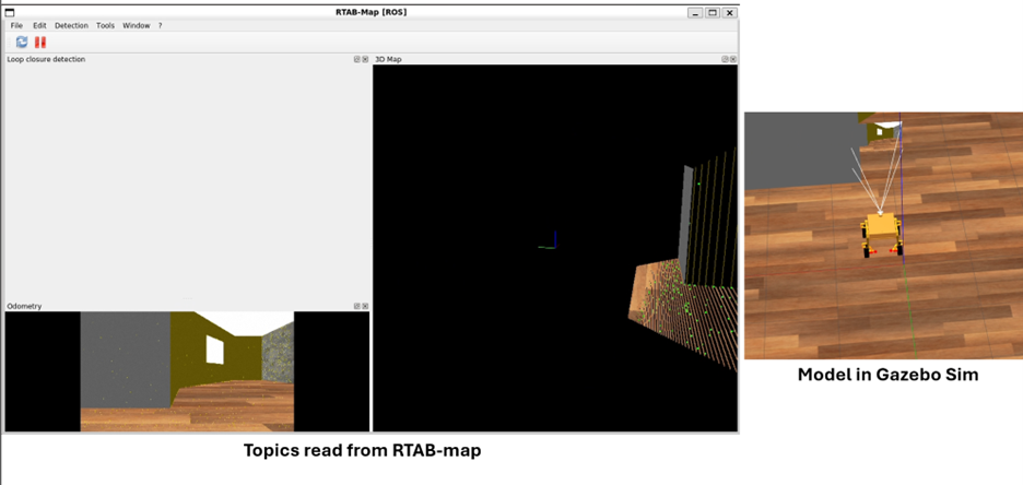
The simulated environment allowed us to test the functionality of the Xbox Controller's mappings and translate the controls over to manual drive commands before actual hardware drive tests, although still lacking the communication package - this process is depicted below. The simulation was most effective at testing the components of the automation pipeline. We were able to simulate RGB image data, depth image data, and IMU data successfully to test that RTABMAP was built properly and was capable of outputting a cost-map and visual odometry with our software environment. We were also able to test the Extended Kalman Filter in simulation, as the simulated sensors were defined to have gaussian noise and we were able to test the filter's tuning and observe the fusion performance between visual odometry and imu data without hardware. A test of RTABMAP GUI Viewer is depicted below.
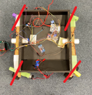
When the rover wasn't available for hardware testing, a pallet rover was constructed to test the autonomy pipeline's functionality while transitioning from Sim2Real. With this, we were able to test that the output drive commands values are expected (a commanded turn left if the rover is getting too close to right wall and vice-versa), as well as a test of obstacle avoidance and collision recovery behaviors before it gets on the actual rover. The testing setup and the 2D generated map is depicted below.

The RealSense camera was initially tested on a personal computer using the standard API provided by Intel. Throught the initial testing, we were able to learn how to take RGB and depth images of various qualities, and how to compress them into a viewable format.
The next round of testing involved the RealSense camera on the NVIDIA Jetson. The camera functionality needed to be integrated with our ROS ecosystem. First, the camera was tested to make sure it was able to take the pictures periodically and save them to disk. Afterwards, the camera was integrated with joystick controls. Thus, the camera needed to be tested in being able to take pictures at the press of a button on the Xbox controller. Finally, the camera was integrated with the Intel RealSense ROS wrapper, and needed to be tested that it can receive raw images at a rate of ~25 FPS and convert them to JPEGs without any lost or missed images.
The mapping pipeline relied on a lot of different tests once images were retrieved from the camera. There were image to mesh tests and file conversion tests. The mapping pipeline operates in a very decoupled manner, it makes sense to split up these tests into chronological occurrences.
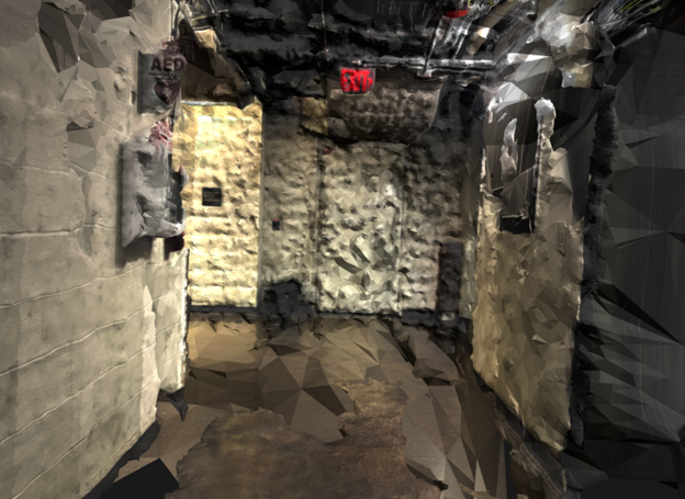
Photogrammetry was carried out through Meshroom, so we needed to test this software and how it worked. Taking images of a figurine with an iPhone yielded promising but distorted results, not good enough to validate use of this program. However, by emulating the rover movement by placing the phone lower and taking pictures of a hallway at left, right, and middle positions produced an extremely accurate map of that environment. Since that raw pipeline worked, more tests were conducted to turn the knobs of the Meshroom nodes to get better outputs. Different filetypes were tested, different meshing techniques, different distortion and mesh filters, different depth map construction parameters were changed, and yet those effects were either minimal or worsened the output, so the raw photogrammetry pipeline in Meshroom was used. Additionally, tests were run with the developer version of Meshroom, especially to explore the option of developing a custom node using pre-existing depth data. Preliminary results with getting a pre-existing depth import node working showed no improvement in mesh output, and further trials with replacing generated depth maps with pre-existing ones resulted in the program crashing. Using this standard photogrammetry pipeline, results were accurate and detailed. Most tests after this point were with the Benedum 4th floor hallway or the Enlow Tunnel on the Montour Trail.
Additionally, two other programs were used to augment the photogrammetry process. Using RTABMAP, a fully textured mesh can be exported from the program, which was worse than the one outputted from Meshroom. However, the input pictures used to construct the point cloud in RTABMAP that would then be reconstructed into a textured mesh could be exported, leaving an image dataset that can be ran entirely in Meshroom's photogrammetry pipeline. This fusion of RTABMAP image export and Meshroom's entire reconstruction pipeline is what yielded the best results, however the compute requirements for this fusion were way beyond what was onboard the rover. In addition to this option, another test was run using the Meshroom point clouds, exported from the StructureFromMotion node, and then imported into Meshlab, where manual filtering and poisson reconstruction could be added. This yielded less detailed but more uniformly accurate results, as opposed to the all-or-nothing nature of Meshroom. Meshroom tended to give the most detailed and accurate maps, although the results were not uniform and highly dataset dependent, causing holes and untextured sections to remain in the map.
The tests for converting output files were quite conclusive and quick. Using the Blender Python API to run blender in the background and follow the scripted commands, any multiple file OBJ, MTL, and texture file can be loaded into Blender and be outputted as a GLTF file. The mesh is imported, the texture is toggled on, and then the GLTF is exported from Blender to be used in viewing software. This test was developed as a sequence of events in Blender, then converted into a python script, and finally can be ran from a single command to point at mesh files and output a singular textured mesh file at a specified location. This test was very short, but it had been tested on classic Meshroom outputs, along with Meshlab and RTABMAP outputs and it worked consistently.
Once the CAVeBoard PCB was proven to be programmable, we could move on to testing some of the peripherals in conjunction with it. This began by placing the PCB in the V1 test chassis and connecting the steering servos to their respective pins. The board was then programmed with code to turn the servos to a random angle. Successful completion of this verified that the servo level shifters on the PCB were functional using the low-level control code written originally for the STM32-based development board.
Next, the motors were similarly wired up, and the PCB was flashed with a new program to spin the motors at a slow speed. Successful completion of this verified that the motor drivers on the PCB were also functional using the low-level control code written originally for the STM32-based development board.
Finally, the Double Ackermann Steering System was tested using a similar procedure to the Low-Level Control module UART and motor and servo tests. A PC with a TTL serial adapter was used to send arbitrary CAVeTalk movement commands to the board. Each movement command was plugged into a spreadsheet to calculate the individual wheel speeds and steering angles. Using the procedures described in the Low-Level Control module tests, the wheel speeds and steering angles were measured again and checked against the values calculated using the spreadsheet. These tests indicated the steering system was working as expected.
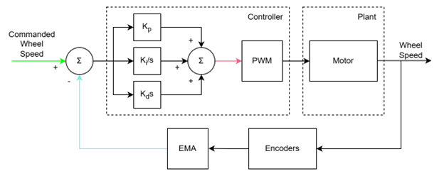
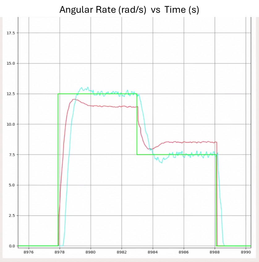
A combination of the Ziegler-Nichols method and manual adjustments were used to tune the PID controller for wheel speed. A series of step inputs was commanded using manual control while the High-Level Control module was used to plot the commanded wheel speed, output of the PID controller, and measured wheel speed. The CAVeTalk configuration messages were used to adjust the PID gains according to the Zeigler-Nichols method to initially stabilize the system. Manual adjustments were then made until overshoot was within 0.5 rad/s and rise time was less than 1s. The result is shown in the plot below, with commanded wheel speed shown in green, the output of the PID controller shown in red, and the measured wheel speed shown in blue.
Manual control tests were performed in two stages: indoor and outdoor tests. During these tests, we confirmed the collective working of the NVIDIA Jetson, MCU, PCB, and rover body. In the initial stage of testing, we drove the rover around the fourth floor of Benedum, using the Xbox controller to communicate to the Jetson, which then sent movement data for the motor controller to execute. Testing on the fourth floor was quite successful, as we were able to drive the rover throughout the halls.
In the next stage of testing, we took the rover to Schenley Park to drive on dirt and gravel terrain. Testing outdoors was a bit more difficult, due to the lack of decent monitors and Wi-Fi. The rover drove successfully on dirt terrain, being able to descend and ascend the Panther Hollow Trail. We also tested driving the motor on gravel terrain at the Schenley Train Tunnel. This terrain proved more difficult to drive on due to the extremely uneven surface. During the gravel tests, the motor joint broke off from one of the rover legs. At the time, we were still using the V1 CAVEMAN rover, which was not as robust as our second iteration.
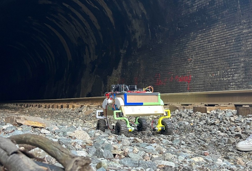
Autonomous control tests followed a similar arc to the manual control tests. First, we performed indoor tests, then transferred to outdoor testing the Enlow Tunnel. Autonomous control tests consisted of everything from manual control tests except for the custom RealSense API (due to lack of compute power during the automation), with the addition of autonomy: the NVIDIA Jetson, MCU, PCB, and rover body. During these tests, the rover was left to autonomously explore after setting autonomous mode, as well as arming the motors using the controller.
The indoor automation tests were successfully able to meet a semi-autonomous state, as it was capable of avoiding collision into walls, avoiding obstacles, as well as turning the sharp corners of Benedum floor 4.
The challenges that we were facing with automation stems from still, a lack of compute power and insufficient I/O bandwidth. The Jetson AGX Xavier's ports we're limited, and the RealSense Camera was enumerated as a USB 2.1 device regardless of whether it was on a USB hub, or directly plugged into a port, which bottlenecked the data transmitted over USB. This, combined with the limited compute power, caused RTABMAP to miss critical frames that it needs for feature-matching, localization, and map generation - as it only outputs after recognizing enough correspondences between frames. As a result, the rover would occasionally pause, as RTABMAP lost its localization, and would need a while to recover. Our workaround to this issue was to simply drive the rover as slow as possible.
After indoor testing, we took the rover to the Enlow Tunnel to perform outdoor tests. Autonomous testing at the Enlow Tunnel was also successful, with the rover being able to drive through the tunnel independently without running into the tunnel walls.
The maximum speed reached during both indoor and outdoor autonomous tests was ~0.5 m/s.
The map generation tests relied on taking the images after a full manual test and creating a mesh from them. The main test was seeing if the 10s of thousands of images could be easily converted into a textured mesh within a reasonable amount of time and with high accuracy and detail. The first experiment after a manual test involved putting 20,000 images into the mapping pipeline, where it took 3 days to run and the output was moderately detailed but had heavy distortions. The same dataset was then used as a basis for pruning, where the perceptual hashing and crop-resistant perceptual hashing techniques were employed. The basic test procedure was running the duplication detection and cutting algorithm on all of the images and then putting the remaining images through the pipeline. The first iteration relied on binning the images, then going through each bin and finding the least blurry similar image. This process was on the order of O(4n), but all the computer vision techniques also relied on the image dimensions, so the runtime was high. The crop resistant technique operated similarly, but the runtime went up by 2-3x without much output improvement. Overall, these hashing techniques did marginally reduce the runtime performance of the photogrammetry pipeline, and the cost of this pre-processing was high. These pruning techniques did not shrink the dataset enough to be of any long-term value, so the best bin sampling approach was used. Testing this technique, we produced our best maps, and it makes sense, as we are basically cutting the stream of frames outputted from the camera into keyframes, similar to what would be taken by hand. This method was optimized for photogrammetry, which made it our best pruning technique for our dataset.
Much of the manual driving was done around the 4th Floor of Benedum, with the rover being controlled with an XBOX controller and making laps around the floor in the span of 3-5 minutes for a full loop. This testing included steering and speed tests on smooth terrain, driving over rough objects and around obstacles, and testing communication sanctity. There were numerous driving tests to ensure robustness, maneuverability, and because it was fun to drive around the rover. These tests collected many images, using many different versions of low- and high-level control running on it. Manual testing allowed us to calibrate the rover with maximum speed and control the steering angle that would provide the highest handling without compromising the mechanical integrity of the rover. These tests also allowed the low-level control to iterate and refine its kinematic modeling, along with testing and controlling different aspects of the rover under full and partial loads. Manual testing lets us see power distribution issues which tended to manifest as communication errors, as the low- and high-level controls tended to get out of sync after a long time. There were many attempts at debugging this issue but due to time constraints, these remain largely unhandled. The high level control was also iterated with these tests, ensuring that human control was straightforward, such that simulation and subsequently autonomous control could transition in seamlessly. The camera capture node was vastly improved through manual testing as the mapping pipeline demanded more image inputs, forcing the camera capture node to optimize its outputs and on-the-fly image compression. The mapping pipeline used all this data to improve its accuracy, as the reference for the maps was easily accessible such that the map parameters could be consistently tuned to ensure the output matched the input.
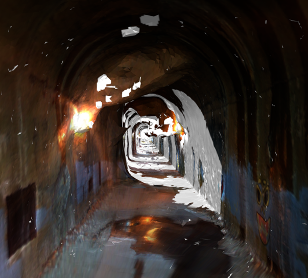
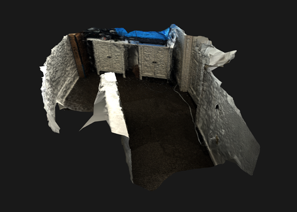
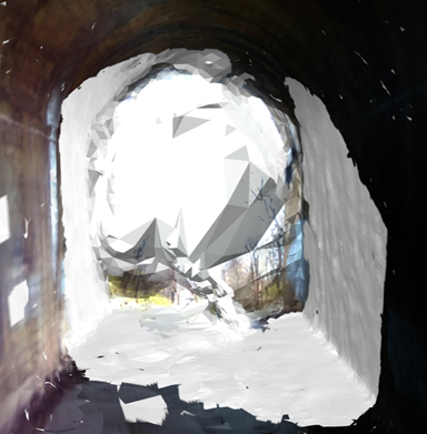
The testing at the Enlow Tunnel was our culminative manual test, as it allowed us to capture many images, driving and following the rover closely behind, and gain a new reference of maneuverability and mapping. Operating the rover at near freezing temperatures also allowed us to gauge the robustness of the system, and the rover even experienced snow. Despite these weather conditions, the rover drove well, at a top speed of 1.5 m/s and let us create accurate maps. Further manual tests determined that the resilience of the suspension and the high torque motors were perfect for getting over rough terrains. These manual tests assured us that the rover we created could handle tough environments, light up dark areas, and create accurate maps as an end-to-end system.
Under manual driving, this was the best map that was created. Other maps that were created from this test can be seen in previous sections.
Like the manual driving tests, the autonomy tests we're first tested on the 4th floor of Benedum and successfully avoided walls and obstacles. We were able to move on to an outdoor autonomy test at the Enlow tunnel with successful autonomous driving slowly as well. Unfortunately, due to the limited computational power of the onboard processing for autonomy, the camera node could not be active at the same time that the autonomous driving was running, and thus the standard inputs of the mapping pipeline could not be collected. Thus, there is no generated 3D map to show for the autonomous driving tests.
Despite our roadblocks in successful, one-shot autonomy on the Jetson Xavier AGX, we're hopeful for the future of our automation pipeline. Our tests on a higher-power AMD64 laptop was capable of vastly superior localization performance, as the RealSense camera was functioning at full performance, and the hardware on the laptop was capable of feature-matching far quicker, essentially never resulting in a loss of correspondences.
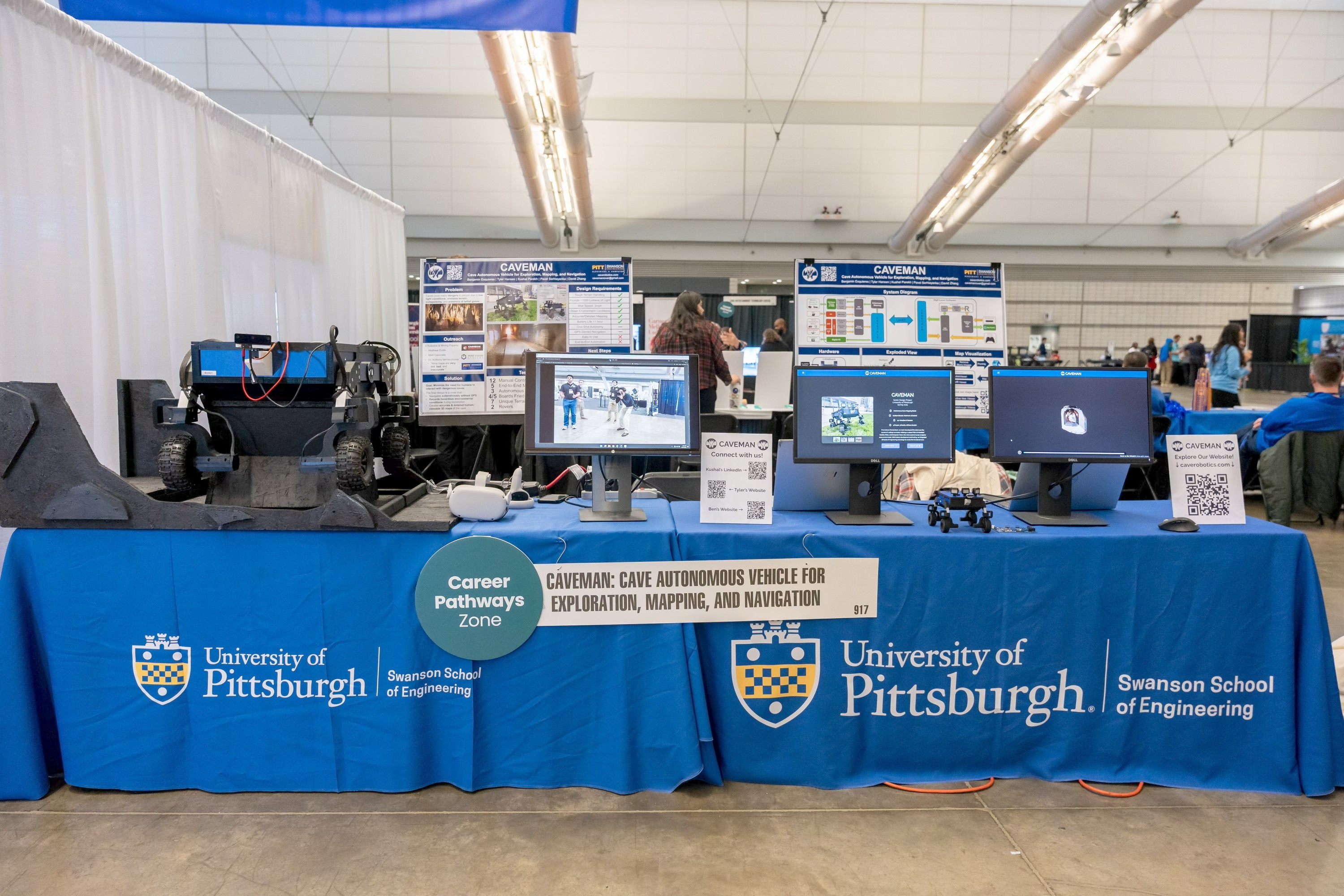
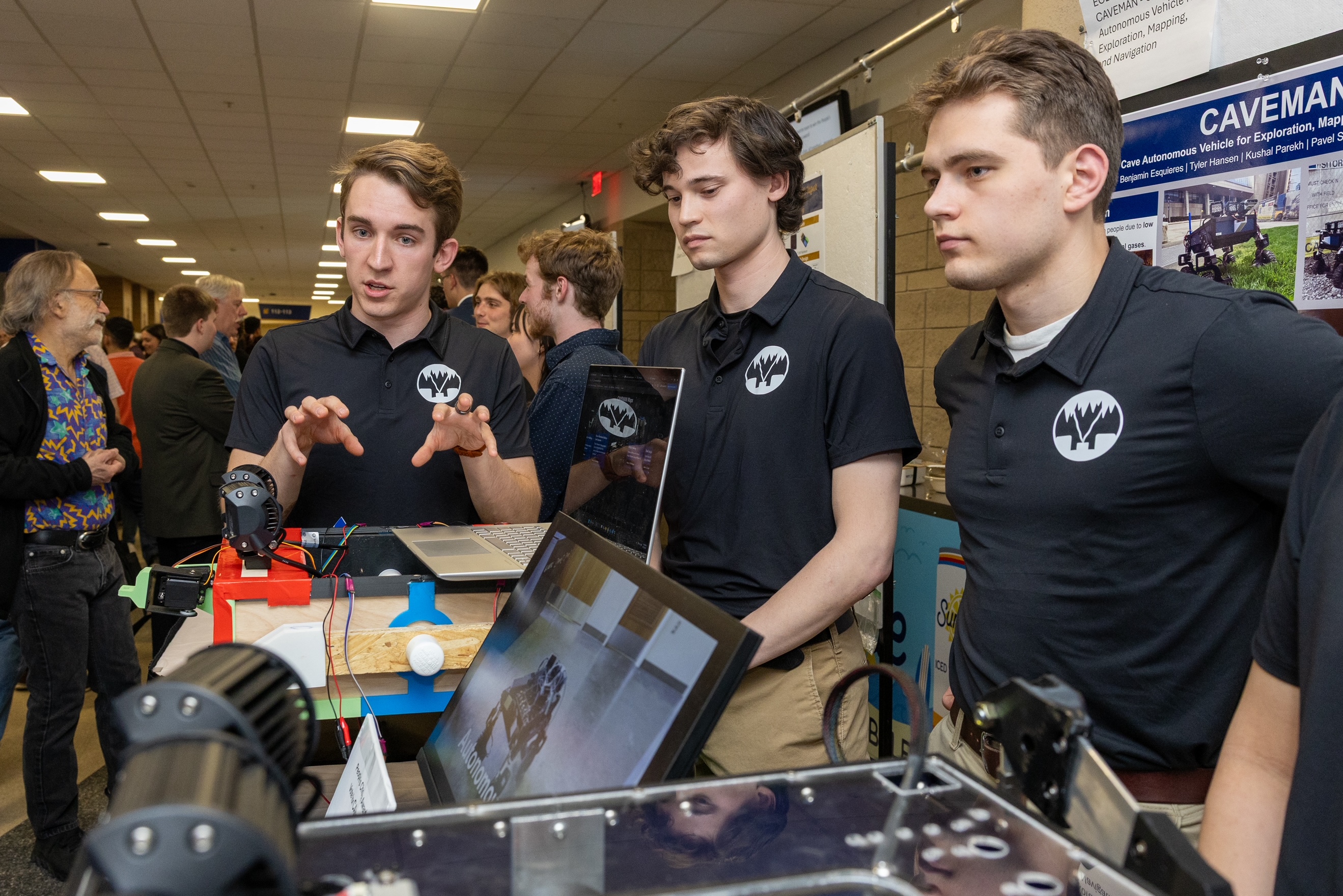
Design Expo Spring 2025
In mid-April, we presented our work at the Spring 2025 Pitt SSOE Design Expo, winning 3rd overall in the ECE Department. We were very happy to show off all the work and love that went into this project, especially since our advisor put a lot of faith in us to pull it all off. Luckily, this project isn't fully done yet, as we have more plans and presentations in store. We planned to rework the system for demoing at Pittsburgh Robotics Network Robotics and AI Discovery Day.

CAVEMAN Rework: New Hardware, Software, Virtual Reality Platforms
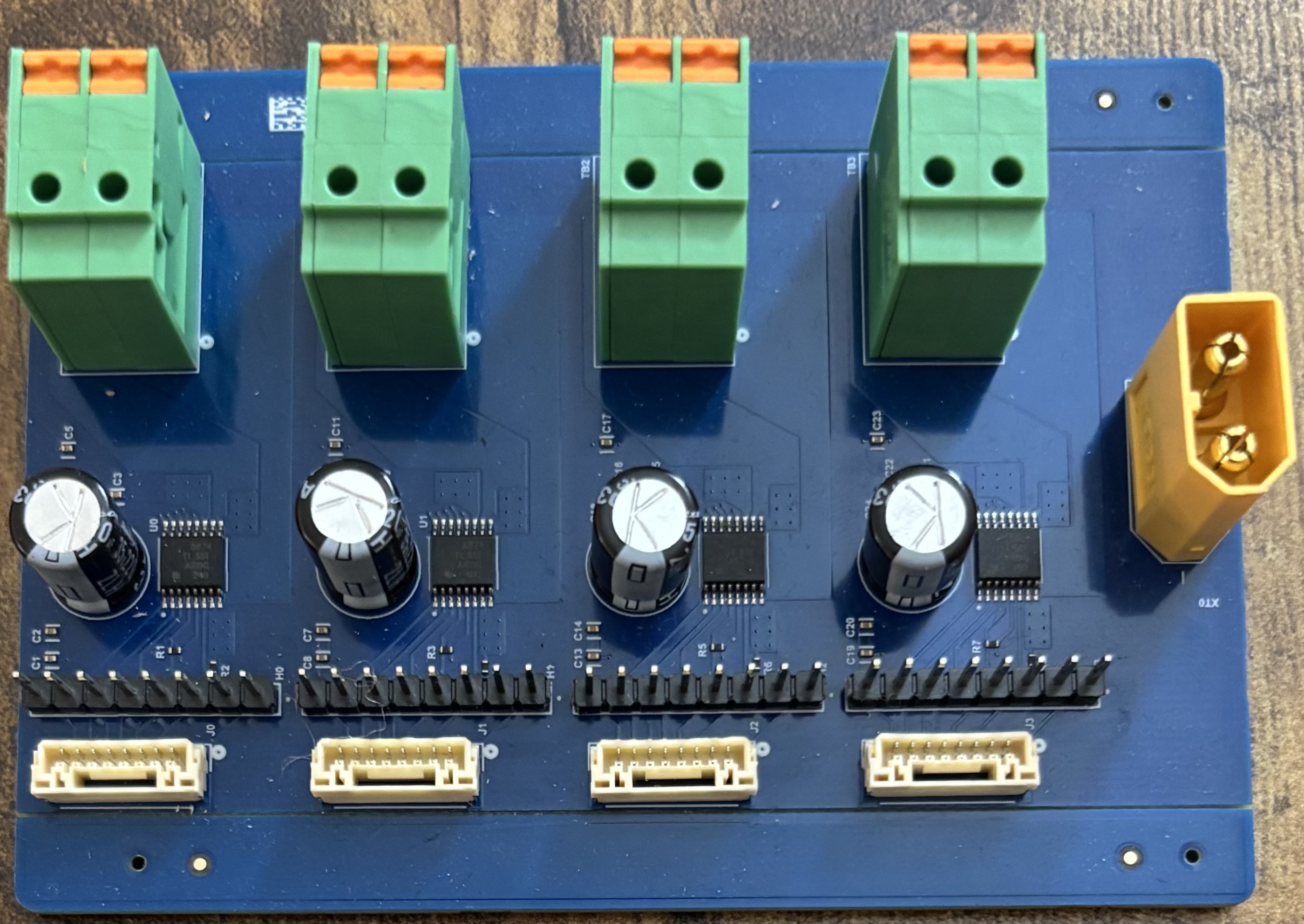
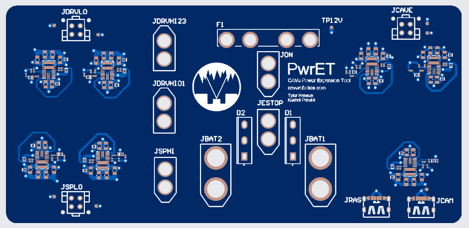
After spending the summer cooling off and making this website as documentation, we started progress towards a CAVEMAN rework. Having one large PCB tailored for CAVEMAN, while successful for the main project, is not sustainable for iteration. Small reworks require fully new PCB manufacturing, compounding costs exponentially. Through this rationale, we split up the main PCB into a computational board, power board, and servo-motor board. Splitting up the PCB this way allows individual debugging of separate boards to ensure certain subsystems are correct and can be fixed while minimizing redundant manufacturing. In addition to this change, we moved our high-level software stack from the Nvidia Jetson to a Raspberry Pi 4. This change was justified due to borrowing and returning the Jetson to the ECE Department, not needing autonomy for demos, and having the RPi 4 readily at hand. The final change was integrating a new depth camera into CAVEMAN and adding a VR teleoperation platform to manually control the system.
Splitting the CAVeBoard into 3 distinct PCBs had the additional purpose of reuse for new projects. By splitting up the main computational board into standalone hardware, it can be adapted to other vehicles, such as underwater robots or drones. This also allows the other boards to be mixed and matched to suit different needs. The power board is necessary for all systems but it can be adjusted to any battery form factor for weight tradeoffs. The servo-motor board has all the high-voltage and high-current peripherals that caused voltage spikes near the computational modules in the original board. By separating and decoupling these systems on different boards, we aimed to increase modularity and resilience while decreasing manufacturing costs. To keep these boards extensible for new projects, more uniform connectors were used to streamline interfacing. More pins were also exposed, lending itself to a devboard design.
Improved software stacks for low and high level functionality were developed during this rework. The low-level software got improvements that made it more portable to other ST microcontrollers such that when the Brain PCB, the old CAVeBoard, or a new MCU was used, the same stack could be utilized. Porting over the high-level functionality was straightforward as we dropped the use of ROS2 in favor of SDL2. Since these new developments were purely for demo purposes, the autonomy stack was not important meanwhile responsive manual control was extremely necessary. SDL2 has event-based polling as opposed to ROS2's timing-based polling, making it more conducive to better performance. Since a new high-level computer was used, we got to test and improve on the extensibility of CAVeTalk. The performance on the Raspberry Pi 4 was similar to the Nvidia Jetson, including the presence of the transmission resets/blackout. This bug still plagued the system on this new platform, pointing to either issues in CAVeTalk's implementation, such as thread-safety, or in the hardware itself.
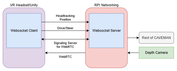
The flashiest part of this rework was implementing VR teleoperation. On the RPI4, we set up a few websocket servers. The main one was for signaling to establish a WebRTC connection between the VR headset and the RPI4, allowing data to be streamed from CAVEMAN into the VR landscape. The other websockets were for sending VR control states, like headset quaternions and controller commands, to the RPI4 to operate CAVEMAN. The VR capabilities included built-in headtracking, mapping headset orientation to the rover's camera servos. Along with that, the VR controllers were used to drive and steer the rover. The VR-side of the system was created in Unity, using WebRTC and Websockets in C# to establish and maintain the connection, plastering the received frame on a camera-locked canvas. The RPI4 uses a mix of Python and C++ to send and receive signals and data accordingly. By the end of all this, we had successfully revived CAVEMAN and added a brand-new feature to its capabilities. New hardware, software, and teleoperation were ready for Robotics and AI Discovery Day.
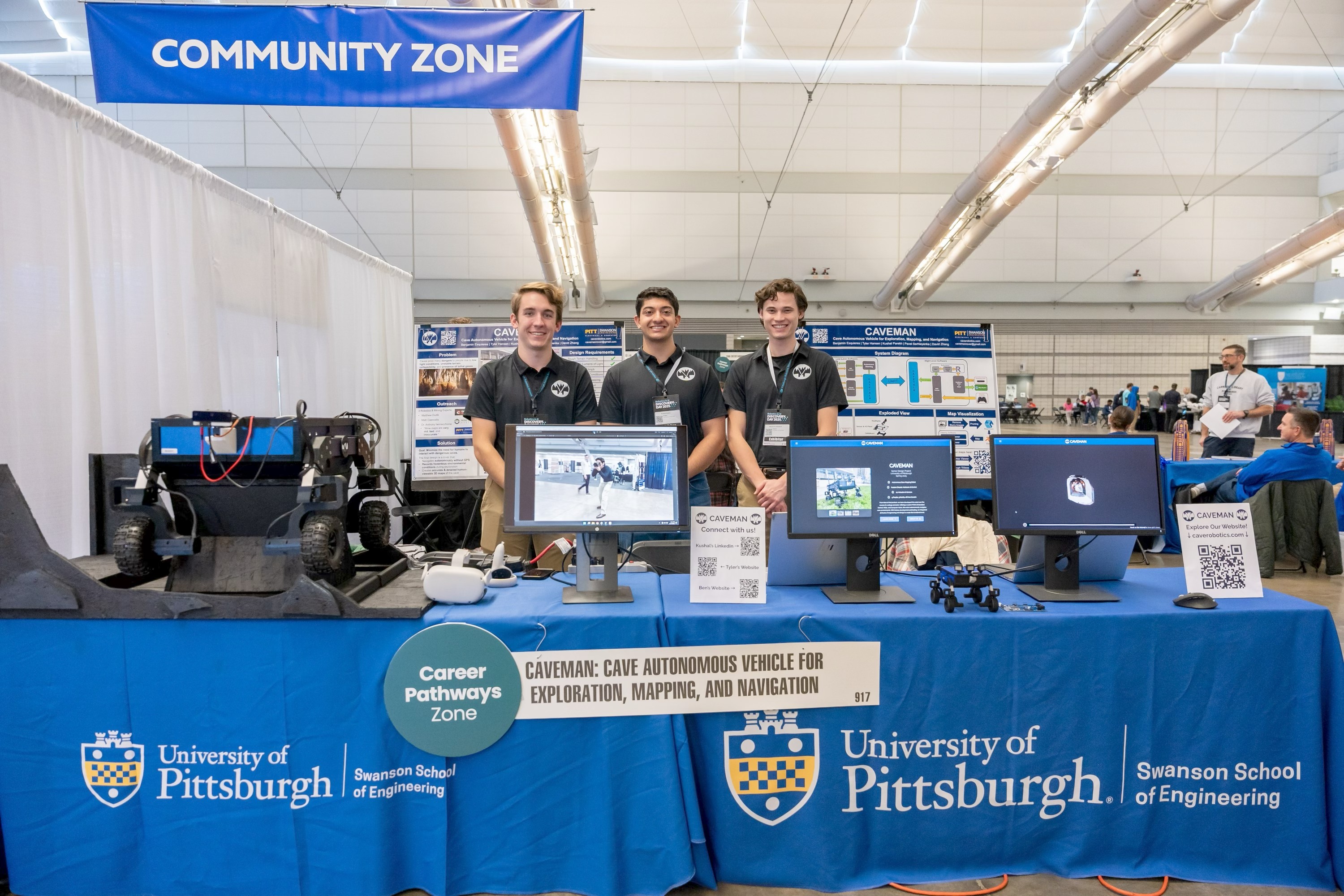
Pittsburgh Robotics Network Robotics & AI Discovery Day
After setting up our booth at RADD the day before, we spent the 9 hours of the convention showing off our project. We let robotics enthusiasts of all ages test out our VR system, particularly our head tracking, along with explore our original maps and website. We also were able to show off our posters and talk to people and investors about our process and further prospects. While this project was fundamentally out of passion, being able to have people test our system and give real feedback was extremely validating, along with talking about our development experience with people who had similar experiences. We had a great amount of fun at Pittsburgh Robotics Network's 2025 Robotics and AI Discovery Day, and we had so much fun with CAVEMAN. We look forward to the next chapter of CAVEMAN.